Lesson 7: Transformers, Attention & Pre-trained Models
Learning Objectives
- Understand the limitations of RNNs and why attention was invented.
- Explain self-attention and how Transformers process sequences in parallel.
- Compare BERT (bidirectional) vs GPT (autoregressive) architectures.
- Use pre-trained models for downstream NLP tasks.
Recap: From Embeddings to Sequences
In Lesson 6 we learned to map tokens → embeddings. But how do we model order and context?
digraph sequence_problem {
  rankdir=LR;
  node [fontsize=11, shape=box, style=rounded];

  t1 [label="The"];
  t2 [label="cat"];
  t3 [label="sat"];
  t4 [label="on"];
  t5 [label="the"];
  t6 [label="mat"];
  q  [label="???"];

  t1 -> t2 -> t3 -> t4 -> t5 -> t6 -> q [style=dashed];
}
- Mean pooling loses word order (e.g., "dog bites man" vs "man bites dog").
- We need models that understand sequential dependencies.
RNNs & LSTMs: The Sequential Approach
- RNNs process tokens one at a time, maintaining a hidden state.
- LSTMs add gates to better capture long-range dependencies.
- Problem: sequential processing is slow (no parallelism).
- Problem: long sequences still cause gradient issues.
digraph rnn {
  rankdir=LR;
  node [fontsize=10, shape=circle];

  h0 [label="h₀"];
  h1 [label="h₁"];
  h2 [label="h₂"];
  h3 [label="h₃"];
  hn [label="h_n"];

  x1 [label="x₁", shape=box];
  x2 [label="x₂", shape=box];
  x3 [label="x₃", shape=box];
  xn [label="x_n", shape=box];

  h0 -> h1 -> h2 -> h3;
  h3 -> hn [style=dashed];
  x1 -> h1;
  x2 -> h2;
  x3 -> h3;
  xn -> hn;
}
The Attention Intuition
Instead of compressing everything into one hidden state, let the model look back at all previous tokens.
- "Attention" = learned soft lookup over a sequence.
- Originally designed for machine translation (Bahdanau et al., 2015).
- Allows focusing on relevant words regardless of distance.
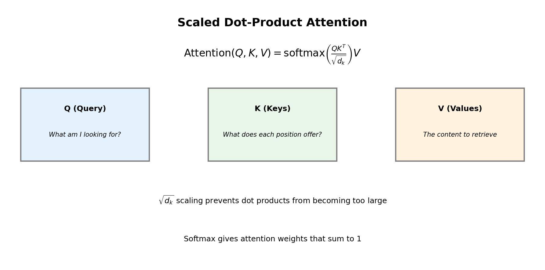
Attention as Soft Dictionary Lookup
Think of attention like a fuzzy database query:
- Query (Q): "What am I looking for?" — current position's representation.
- Keys (K): "What does each position offer?" — representations of all positions.
- Values (V): "What information to retrieve?" — content at each position.
\[ \text{Attention}(Q, K, V) = \text{softmax}\left(\frac{QK^\top}{\sqrt{d_k}}\right) V \]
The \(\sqrt{d_k}\) scaling prevents dot products from becoming too large.
Dot Product as Similarity Measure
Why do we use \(QK^\top\) to compute attention scores?
- High dot product: vectors point in similar directions → high similarity.
- Zero: orthogonal vectors → no relationship.
- Negative: opposite directions → dissimilar.
In attention: \(Q_i \cdot K_j\) measures how much position \(i\) should attend to position \(j\).
Attention Formula Explained
- Step 1: Compute similarity scores: \(QK^\top\) (dot product of queries and keys)
- Step 2: Scale by \(\sqrt{d_k}\) to prevent gradient vanishing/exploding
- Step 3: Apply softmax to get attention weights (sum to 1)
- Step 4: Weight the values and sum to get context-aware representations
Attention Data Flow
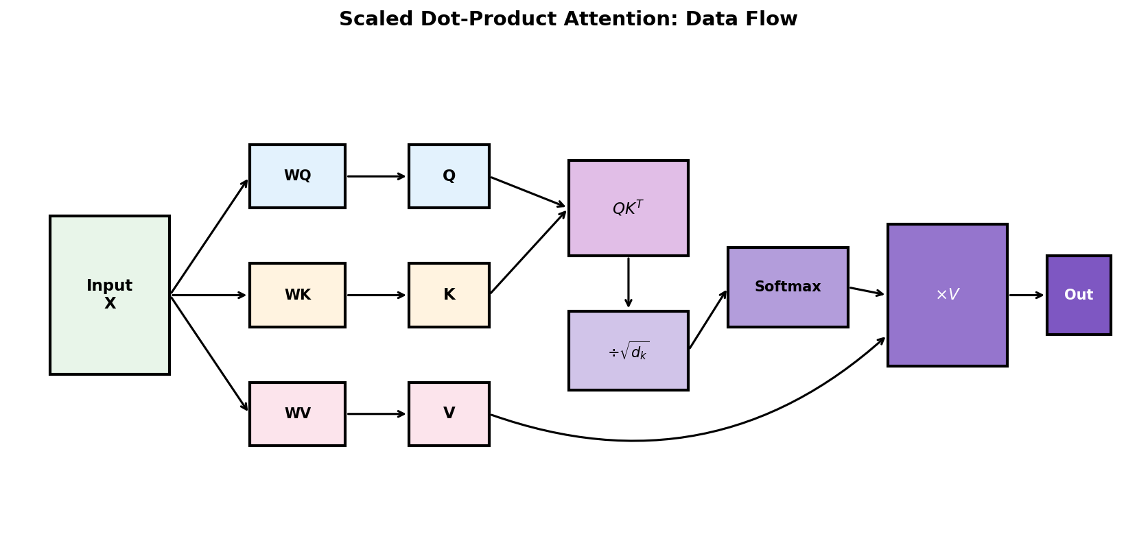
- Project input X to Query, Key, Value matrices using learned weights
- Compute attention scores: \(QK^T\) measures similarity between all pairs
- Scale by \(\sqrt{d_k}\) to stabilize gradients
- Softmax normalizes scores to sum to 1 (attention weights)
- Weight values by attention and sum → context-aware output
Why Scale by \(\sqrt{d_k}\)?
The scaling factor prevents numerical instability:
Problem without scaling:
- If \(d_k\) is large (e.g., 512), dot products can be very large.
- Large values → softmax saturates → gradients vanish.
- Example: \(e^{100} \approx 10^{43}\) dominates everything else.
With scaling:
- Dividing by \(\sqrt{d_k}\) keeps values in a reasonable range.
- Softmax outputs remain smooth (not 0/1).
- Gradients flow properly during training.
Intuition: If Q and K entries are ~unit variance, their dot product has variance ~\(d_k\). Scaling restores unit variance.
Self-Attention: Attending to Yourself
In self-attention, Q, K, and V all come from the same sequence.
digraph selfattn {
  rankdir=TB;
  node [fontsize=10, shape=box, style=rounded];

  input [label="Input Embeddings\n[x₁, x₂, x₃, x₄]"];
  wq [label="Wq"];
  wk [label="Wk"];
  wv [label="Wv"];
  q [label="Queries (Q)"];
  k [label="Keys (K)"];
  v [label="Values (V)"];
  attn [label="Attention Scores\nsoftmax(QKᵀ/√d)"];
  out [label="Weighted Values\nContext vectors"];

  input -> wq -> q;
  input -> wk -> k;
  input -> wv -> v;
  q -> attn;
  k -> attn;
  attn -> out;
  v -> out;
}
Each token can attend to every other token — capturing long-range dependencies in one step!
Visualizing Self-Attention
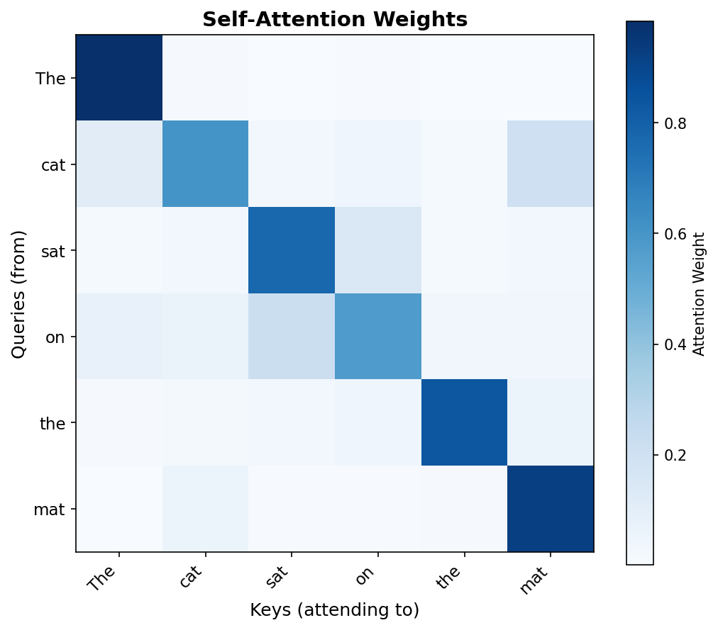
Reading the heatmap:
- Rows = queries (which word is "asking")
- Columns = keys (what it's attending to)
- Darker = higher attention weight
- Each row sums to 1 (softmax)
The model learns to focus on semantically related tokens — capturing context without recurrence!
Multi-Head Attention: The Intuition
Why use multiple attention heads instead of one?
- "The cat that I saw yesterday was sleeping"
- Syntactic: "cat" ↔ "was" (subject-verb agreement)
- Semantic: "cat" ↔ "sleeping" (who is sleeping?)
- Positional: "cat" ↔ nearby words
- Solution: Run multiple attention operations in parallel, each learning different patterns.
What is \(d_k\)? Dimension of Keys
In multi-head attention, we split the model dimension across heads:
- \(d_{model}\) = total embedding dimension (e.g., 512, 768, 1024)
- \(n_{heads}\) = number of attention heads (e.g., 8, 12, 16)
- \(d_k = d_v\) = dimension per head
| Model | \(d_{model}\) | \(n_{heads}\) | \(d_k\) |
|---|---|---|---|
| Transformer (original) | 512 | 8 | 64 |
| BERT-base | 768 | 12 | 64 |
| GPT-2 small | 768 | 12 | 64 |
| GPT-3 (175B) | 12288 | 96 | 128 |
How \(d_k\) is Used: Step by Step
Multi-head attention reshapes tensors to give each head its own \(d_k\)-dimensional subspace:
# 1. Start with input: (batch, seq_len, d_model)
x.shape  # (32, 100, 768)

# 2. Project to Q, K, V using linear layers
Q = W_q(x)  # (32, 100, 768) — still full dimension

# 3. Reshape: split d_model into (n_heads, d_k)
Q = Q.view(batch, seq_len, n_heads, d_k)  # (32, 100, 12, 64)
Q = Q.transpose(1, 2)                      # (32, 12, 100, 64)
#         ↑ now each of 12 heads has 64-dim vectors

# 4. Compute attention PER HEAD
scores = Q @ K.transpose(-2, -1)  # (32, 12, 100, 100)
scores = scores / math.sqrt(d_k)  # divide by √64 = 8

# 5. Concatenate heads back
output = output.transpose(1, 2).reshape(batch, seq_len, d_model)
Key insight: The \(\sqrt{d_k}\) scaling uses the per-head dimension (64), not the full model dimension (768).
What is a "Head" Exactly?
Each head is an independent attention computation with its own learned projections:
Each head has:
- Its own \(W_Q^{(i)}\), \(W_K^{(i)}\), \(W_V^{(i)}\) matrices
- Its own \(d_k\)-dimensional subspace
- Its own attention pattern to learn
Mathematically:
Where \(W_Q^{(i)} \in \mathbb{R}^{d_{model} \times d_k}\)
Think of it as: Each head "looks at" the input from a different angle, like multiple experts examining the same data.
How Heads are Combined
After computing attention in parallel, heads are concatenated and projected:
# Each head outputs: (batch, seq_len, d_k)
head_outputs = [head(Q, K, V) for head in heads]  # list of 12 tensors

# Concatenate along last dimension
concat = torch.cat(head_outputs, dim=-1)  # (batch, seq_len, 12*64=768)

# Final projection mixes information across heads
output = self.W_o(concat) # (batch, seq_len, 768)- Concat: Each head contributes \(d_k\) dimensions → total \(n_{heads} \times d_k = d_{model}\)
- \(W_O\): Learns how to combine information from all heads
What Do Different Heads Learn?
Research has shown heads specialize in different linguistic phenomena:
| Head Type | What It Learns | Example |
|---|---|---|
| Positional | Attend to previous/next token | Bigram patterns, local context |
| Syntactic | Subject-verb, noun-adjective | "cats" → "are" (agreement) |
| Coreference | Pronouns to their referents | "it" → "the cat" |
| Semantic | Meaning-based relations | "doctor" → "hospital" |
| Delimiter | Attend to [CLS], [SEP], punctuation | Sentence boundaries |
Visualizing Head Specialization
Different heads in BERT attend to different patterns:
Head A: Positional
The  [███░░░░░]
cat  [░███░░░░]
sat  [░░███░░░]
on   [░░░███░░]
the  [░░░░███░]
mat  [░░░░░███]
Attends to nearby tokens
Head B: Syntactic
The  [░░░░░░░░]
cat  [░░░░░░░█]  → "sat"
sat  [░█░░░░░░]  → "cat"
on   [░░░░░░░░]
the  [░░░░░░░░]
mat  [░░█░░░░░]  → "sat"
Subject-verb-object links
Multi-Head Attention: Code
class MultiHeadAttention(nn.Module):
    def __init__(self, d_model, n_heads):
        super().__init__()
        self.n_heads = n_heads
        self.d_k = d_model // n_heads
        self.W_q = nn.Linear(d_model, d_model)
        self.W_k = nn.Linear(d_model, d_model)
        self.W_v = nn.Linear(d_model, d_model)
        self.W_o = nn.Linear(d_model, d_model)

    def forward(self, x):
        B, T, C = x.shape
        # Project and reshape: (B, T, C) → (B, n_heads, T, d_k)
        Q = self.W_q(x).view(B, T, self.n_heads, self.d_k).transpose(1, 2)
        K = self.W_k(x).view(B, T, self.n_heads, self.d_k).transpose(1, 2)
        V = self.W_v(x).view(B, T, self.n_heads, self.d_k).transpose(1, 2)

        # Attention per head
        scores = (Q @ K.transpose(-2, -1)) / math.sqrt(self.d_k)
        attn = F.softmax(scores, dim=-1)
        out = attn @ V  # (B, n_heads, T, d_k)

        # Concatenate and project
        out = out.transpose(1, 2).reshape(B, T, C)
        return self.W_o(out)
Multi-Head Attention Patterns
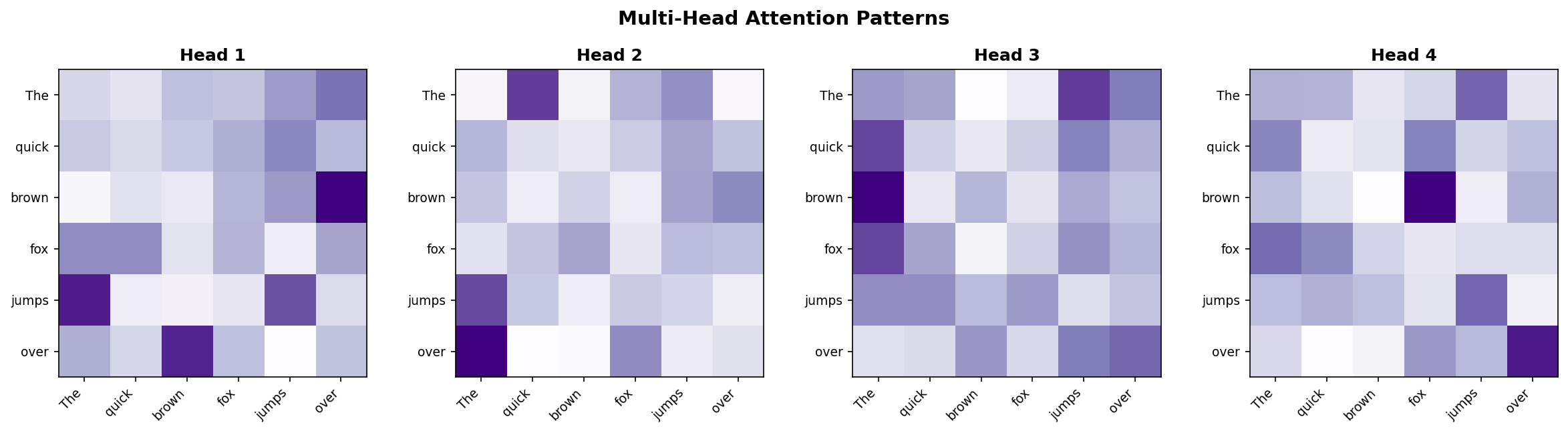
- Different heads, different patterns: Each head attends to different aspects of the input.
- Head 1 might focus on syntactic relations (subject-verb)
- Head 2 might capture semantic similarity
- Head 3 might attend to positional patterns
By combining multiple perspectives, the model builds richer representations.
The Transformer Architecture
"Attention Is All You Need" (Vaswani et al., 2017) — no recurrence, just attention!
digraph transformer {
  rankdir=LR;
  node [fontsize=12, shape=box, style=rounded, height=0.8];
  edge [penwidth=1.5];
  graph [nodesep=0.6, ranksep=1.0];

  input [label="Input Embedding\n+ Positional Encoding"];
  enc1 [label="Encoder Block ×N\n(Self-Attention + FFN)", style="filled,rounded", fillcolor="#e3f2fd"];
  enc_out [label="Encoder\nOutput"];

  tgt [label="Target Embedding\n+ Positional Encoding"];
  dec1 [label="Decoder Block ×N\n(Masked Self-Attn\n+ Cross-Attn + FFN)", style="filled,rounded", fillcolor="#fff3e0"];
  output [label="Output\nProbabilities", style="filled,rounded", fillcolor="#e8f5e9"];

  input -> enc1 -> enc_out;
  tgt -> dec1;
  enc_out -> dec1 [label="Cross-Attention"];
  dec1 -> output;
}
Inside a Transformer Block
Encoder Block
- Multi-Head Self-Attention
- Add & LayerNorm (residual)
- Feed-Forward Network (2 layers)
- Add & LayerNorm
Decoder Block
- Masked Multi-Head Self-Attention
- Add & LayerNorm
- Cross-Attention (to encoder)
- Add & LayerNorm
- Feed-Forward Network
- Add & LayerNorm
Key insight: Residual connections + LayerNorm enable very deep networks.
Transformer Block Architecture
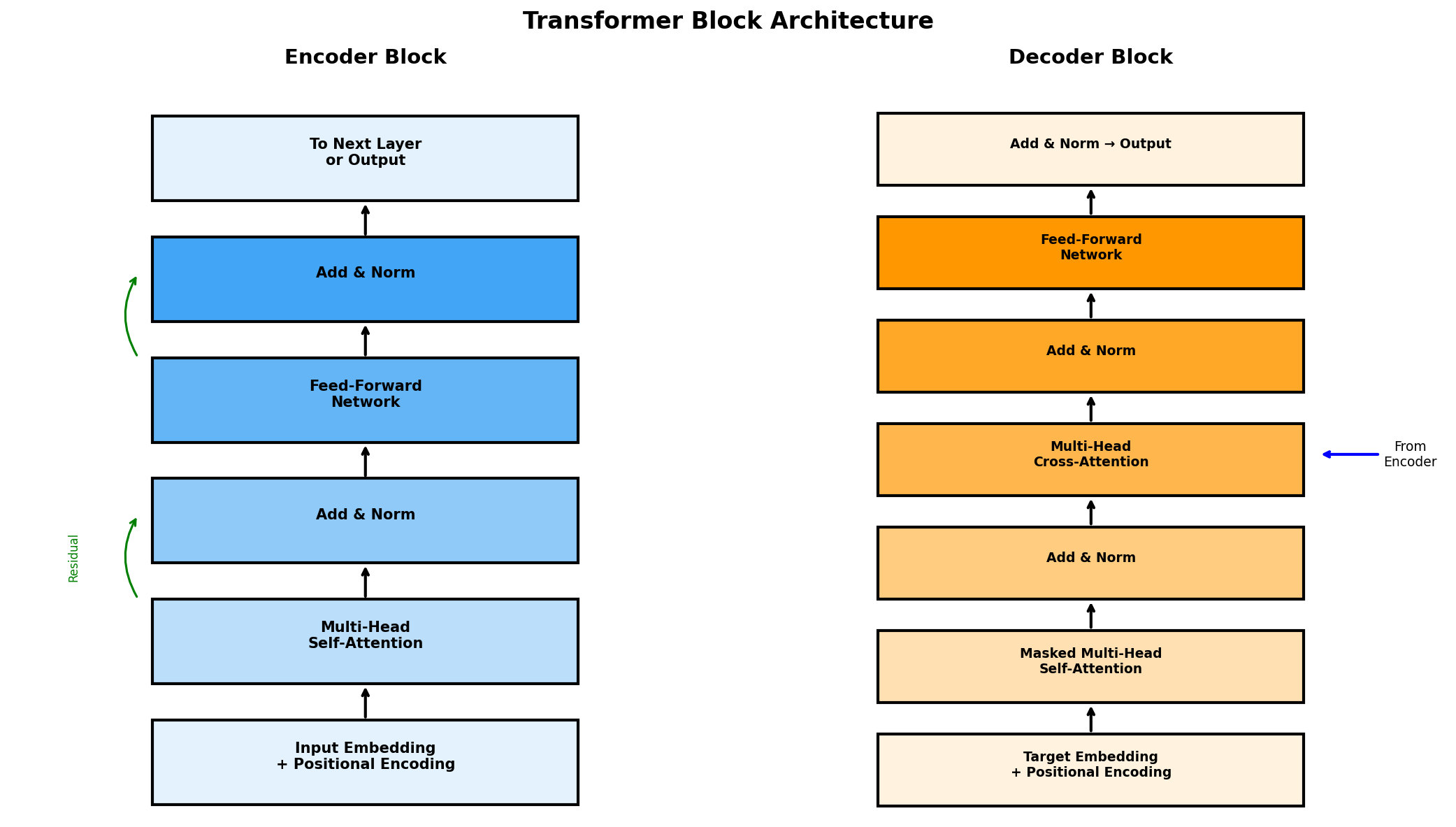
Residual connections (green arrows) allow gradients to flow directly, enabling deep stacking of blocks.
What is Layer Normalization?
LayerNorm normalizes activations across features for each sample independently:
Why LayerNorm (not BatchNorm)?
- Sequences have variable length.
- Works with batch size = 1 (inference).
- Each token normalized independently.
What it does:
- Stabilizes training (prevents exploding activations).
- Reduces internal covariate shift.
- \(\gamma, \beta\) are learnable scale/shift parameters.
Residual Connections Revisited
You've seen these in ResNets (Lesson 4). Same idea here!
- Skip connection: Add input directly to sublayer output.
- Why: Gradients flow through the "+" unchanged → deep networks train.
- Benefit: Sublayer only learns the residual (what to add/change).
# PyTorch pattern
x = x + self.attention(x)    # residual
x = self.layer_norm1(x)      # normalize
x = x + self.feed_forward(x) # residual
x = self.layer_norm2(x)      # normalize
The Feed-Forward Network (FFN)
Each Transformer block has a simple 2-layer MLP applied to each position:
- Expand: Project from \(d_{model}\) to \(4 \times d_{model}\) (typically).
- Non-linearity: GELU (or ReLU in original paper).
- Contract: Project back to \(d_{model}\).
- Applied independently: Same weights, but each token processed separately.
class FeedForward(nn.Module):
    def __init__(self, d_model, d_ff=2048):
        super().__init__()
        self.linear1 = nn.Linear(d_model, d_ff)
        self.linear2 = nn.Linear(d_ff, d_model)
        self.gelu = nn.GELU()

    def forward(self, x):
        return self.linear2(self.gelu(self.linear1(x)))
From Text to Attention: The Full Pipeline
Let's trace how raw text becomes input for attention:
digraph pipeline {
  rankdir=LR;
  node [fontsize=11, shape=box, style=rounded, height=0.6];
  edge [penwidth=1.5];
  graph [nodesep=0.4, ranksep=0.7];

  text [label="Raw Text\n\"The cat sat\""];
  tok [label="Tokenizer", style="filled,rounded", fillcolor="#e3f2fd"];
  ids [label="Token IDs\n[101, 1996, 4937]"];
  emb [label="Embedding\nLookup", style="filled,rounded", fillcolor="#fff3e0"];
  vecs [label="Token Vectors\n(seq, d_model)"];
  pe [label="+ Positional\nEncoding", style="filled,rounded", fillcolor="#e8f5e9"];
  input [label="Transformer\nInput"];
  attn [label="Self-Attention", style="filled,rounded", fillcolor="#ffcdd2"];

  text -> tok -> ids -> emb -> vecs -> pe -> input -> attn;
}
Step 1: Tokenization
Convert raw text into a sequence of token IDs:
# Example with BERT tokenizer
from transformers import BertTokenizer
tokenizer = BertTokenizer.from_pretrained('bert-base-uncased')

text = "The cat sat on the mat"
tokens = tokenizer.tokenize(text)
# ['the', 'cat', 'sat', 'on', 'the', 'mat']

token_ids = tokenizer.encode(text, add_special_tokens=True)
# [101, 1996, 4937, 2068, 2006, 1996, 13523, 102]
#  ↑                                          ↑
# [CLS] [SEP]- Vocabulary: Maps each token to a unique integer ID
- Special tokens: [CLS]=101, [SEP]=102 for BERT
- Subword tokenization: Handles unknown words by splitting
Step 2: Token Embeddings
Look up each token ID in a learned embedding matrix:
# Token IDs → Embeddings
token_ids = [101, 1996, 4937, 2068, 2006, 1996, 13523, 102]
#             ↓     ↓     ↓     ↓     ↓     ↓      ↓     ↓

embedding = nn.Embedding(vocab_size=30522, embedding_dim=768)
token_embeddings = embedding(torch.tensor(token_ids))
# Shape: (8, 768) — 8 tokens, each is a 768-dim vector

# Conceptually:
# [CLS] → [0.12, -0.34, 0.56, ..., 0.78]  # 768 dims
# "the" → [0.23, 0.45, -0.12, ..., 0.91]
# "cat" → [-0.11, 0.67, 0.23, ..., 0.34]
# ...
Each token is now a dense vector in a learned semantic space!
Step 3: Add Positional Encoding
Embeddings alone don't know word order. We add position information:
# Sinusoidal positional encoding
def get_positional_encoding(seq_len, d_model):
    pe = torch.zeros(seq_len, d_model)
    position = torch.arange(0, seq_len).unsqueeze(1).float()
    div_term = torch.exp(torch.arange(0, d_model, 2).float() *
                         (-math.log(10000.0) / d_model))
    pe[:, 0::2] = torch.sin(position * div_term)  # even dims
    pe[:, 1::2] = torch.cos(position * div_term)  # odd dims
    return pe

# Add to embeddings
transformer_input = token_embeddings + positional_encoding
# Shape: still (8, 768)
The Math: Token + Position
Each input vector combines semantic meaning with position:
| Position | Token | Token Embedding | + Pos Encoding | = Input |
|---|---|---|---|---|
| 0 | [CLS] | \(\mathbf{x}_0\) | \(\mathbf{PE}_0\) | \(\mathbf{z}_0\) |
| 1 | the | \(\mathbf{x}_1\) | \(\mathbf{PE}_1\) | \(\mathbf{z}_1\) |
| 2 | cat | \(\mathbf{x}_2\) | \(\mathbf{PE}_2\) | \(\mathbf{z}_2\) |
| 3 | sat | \(\mathbf{x}_3\) | \(\mathbf{PE}_3\) | \(\mathbf{z}_3\) |
| ... | ... | ... | ... | ... |
Now "cat" at position 2 has a different representation than "cat" at position 5!
Step 4: Into Attention
The positioned embeddings become Q, K, V for self-attention:
# Input: positioned embeddings Z = (seq_len, d_model)
Z = token_embeddings + positional_encoding  # (8, 768)

# Project to Q, K, V
Q = Z @ W_q  # (8, 768) @ (768, 768) = (8, 768)
K = Z @ W_k  # (8, 768)
V = Z @ W_v  # (8, 768)

# Compute attention
scores = Q @ K.T / sqrt(d_k)  # (8, 8) — every token attends to every token
weights = softmax(scores, dim=-1)  # (8, 8)
output = weights @ V # (8, 768) — context-aware representationsComplete Data Flow Diagram
| Stage | Shape | Description |
|---|---|---|
| Token IDs | (seq_len,) | Integer indices |
| Embeddings | (seq_len, d_model) | Dense vectors |
| + Pos Encoding | (seq_len, d_model) | Position-aware |
| Q, K, V | (seq_len, d_model) | Projected vectors |
| Attention Scores | (seq_len, seq_len) | Pairwise similarities |
| Output | (seq_len, d_model) | Context-aware repr. |
Positional Encoding Formula
The sinusoidal formula ensures each position has a unique pattern:
- pos = position in sequence (0, 1, 2, ...)
- i = dimension index (0, 1, ..., d/2-1)
- 2i, 2i+1 = even dimensions use sin, odd use cos
- 10000 = base wavelength (larger → slower oscillation)
Why sin/cos? The model can learn to attend to relative positions because \(PE_{pos+k}\) can be represented as a linear function of \(PE_{pos}\).
Visualizing Positional Encoding
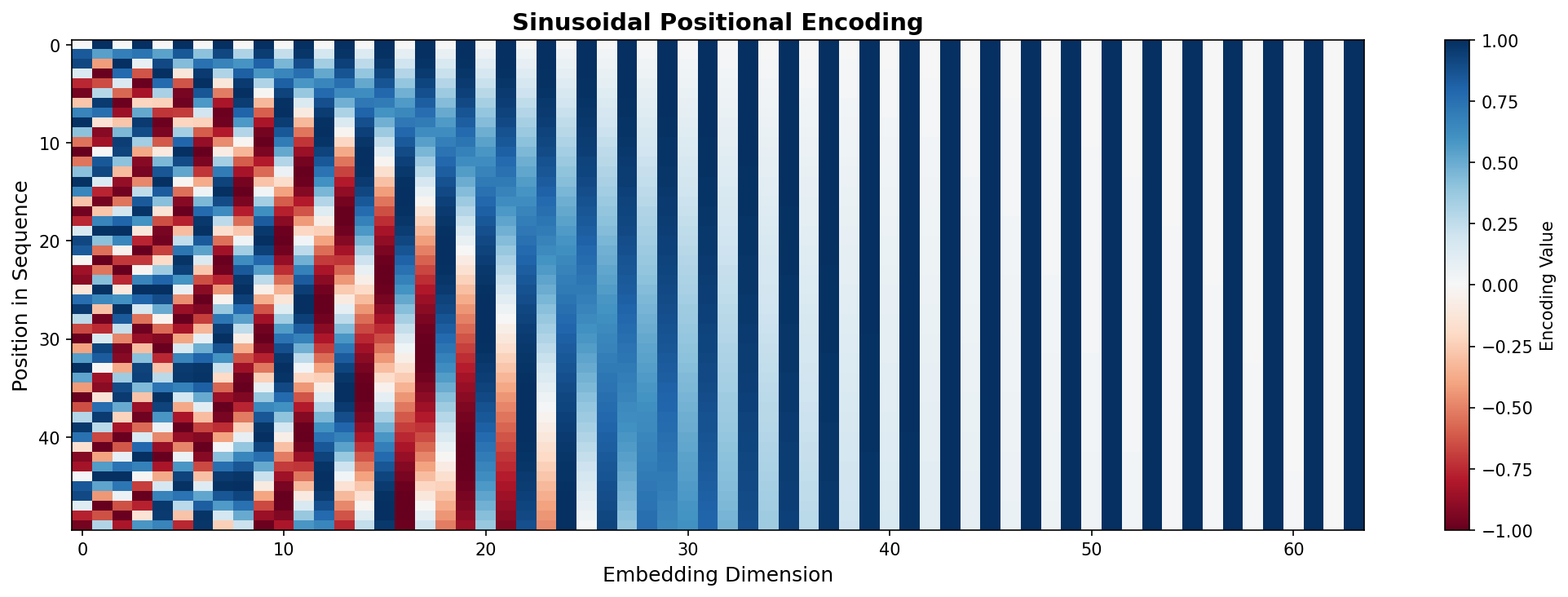
- Y-axis: Position in sequence (0 to 50)
- X-axis: Embedding dimensions (64 total)
- Pattern: Low dimensions oscillate quickly, high dimensions oscillate slowly
- Key insight: Each position has a unique "fingerprint" — the model learns to use these patterns to understand word order.
Self-Attention vs Cross-Attention
Two types of attention in Transformers:
Self-Attention
- Q, K, V all come from the same sequence.
- Each token attends to all other tokens in its own sequence.
- Used in: BERT (encoder), GPT (decoder).
Example: "The cat sat" — each word looks at all words.
Cross-Attention
- Q comes from one sequence (decoder).
- K, V come from a different sequence (encoder output).
- Used in: Encoder-Decoder Transformers (translation).
Example: Translating "Le chat" → decoder queries encoder.
Cross-Attention in Translation
digraph cross_attention {
  rankdir=TB;
  node [fontsize=10, shape=box, style=rounded];

  subgraph cluster_encoder {
    label="Encoder (French)";
    style=filled; fillcolor="#e3f2fd";
    e1 [label="Le"]; e2 [label="chat"]; e3 [label="dort"];
  }

  subgraph cluster_decoder {
    label="Decoder (English)";
    style=filled; fillcolor="#fff3e0";
    d1 [label="The"]; d2 [label="cat"]; d3 [label="sleeps"];
  }

  e1 -> d2 [color=blue, style=dashed, label="K,V"];
  e2 -> d2 [color=blue, style=dashed];
  e3 -> d2 [color=blue, style=dashed];
  d2 -> d2 [label="Q", color=orange];
}
- Decoder position "cat" generates Query.
- All encoder outputs provide Keys and Values.
- Attention finds: "cat" should attend strongly to "chat".
What is Masking?
Masking prevents attention to certain positions:
Padding Mask
- Ignore <PAD> tokens in variable-length sequences.
- Set attention scores to \(-\infty\) for padding positions.
- After softmax: zero attention weight.
Causal (Look-ahead) Mask
- Prevent seeing future tokens during generation.
- Lower-triangular mask: position \(i\) sees only \(j \leq i\).
- Used in GPT and decoder self-attention.
# Causal mask: lower triangular
mask = torch.tril(torch.ones(seq_len, seq_len))
# Apply before softmax
scores = scores.masked_fill(mask == 0, float('-inf'))
Why Does the Decoder Need Masking?
During training, we feed the entire target sequence at once. But we must prevent "cheating"!
Without mask (cheating!):
Input:  "The cat sat on the ___"
Target: "The cat sat on the mat"

Predicting "sat":
  Can see: The, cat, sat, on, the, mat
  ❌ Knows answer before predicting!
With causal mask:
Input:  "The cat sat on the ___"
Target: "The cat sat on the mat"

Predicting "sat":
  Can see: The, cat
  ✅ Must predict from context only!
Key insight: Masking simulates autoregressive generation during parallel training.
Causal Mask: Step by Step
The mask is a lower-triangular matrix that blocks future positions:
The Mask Matrix
        The  cat  sat  on  mat
The   [  1    0    0   0    0 ]
cat   [  1    1    0   0    0 ]
sat   [  1    1    1   0    0 ]
on    [  1    1    1   1    0 ]
mat   [  1    1    1   1    1 ]
1 = can attend, 0 = blocked
After Masking Scores
        The  cat  sat  on  mat
The   [ 0.8  -∞   -∞  -∞   -∞ ]
cat   [ 0.3  0.5  -∞  -∞   -∞ ]
sat   [ 0.1  0.4  0.3 -∞   -∞ ]
on    [ 0.1  0.2  0.3 0.2  -∞ ]
mat   [ 0.1  0.2  0.2 0.1  0.3]
-∞ → 0 after softmax
How \(-\infty\) Masking Works
Setting scores to \(-\infty\) makes them vanish after softmax:
# Before masking: attention scores
scores = [[0.8, 0.5, 0.3, 0.2],   # position 0 attends to all
          [0.3, 0.9, 0.4, 0.1],   # position 1 attends to all
          [0.2, 0.4, 0.7, 0.3],   # position 2 attends to all
          [0.1, 0.2, 0.3, 0.8]]   # position 3 attends to all

# Create causal mask
mask = torch.tril(torch.ones(4, 4))
# [[1, 0, 0, 0],
#  [1, 1, 0, 0],
#  [1, 1, 1, 0],
#  [1, 1, 1, 1]]

# Apply mask: where mask=0, set score to -inf
scores = scores.masked_fill(mask == 0, float('-inf'))

# After softmax: future positions get 0 weight
weights = F.softmax(scores, dim=-1)
Masked Decoder: Training vs Inference
Training (Parallel)
- Feed entire target sequence at once.
- Apply causal mask to prevent cheating.
- Compute loss for all positions in parallel.
- Fast! One forward pass predicts all tokens.
# All predictions at once
logits = model(target_sequence)
loss = F.cross_entropy(logits, target)
Inference (Sequential)
- Start with just [START] token.
- Predict next token, append to sequence.
- Repeat until [END] or max length.
- Slow! One token per forward pass.
# Generate one token at a time
while not done:
    next_token = model(sequence).argmax()
    sequence.append(next_token)
Visualizing Autoregressive Generation
GPT generates text one token at a time, always looking only left:
Step 1: [START] → predicts "The"
        Sees: [START]

Step 2: [START] The → predicts "cat"
        Sees: [START], The

Step 3: [START] The cat → predicts "sat"
        Sees: [START], The, cat

Step 4: [START] The cat sat → predicts "on"
        Sees: [START], The, cat, sat

...continues until [END] token or max length
The causal mask during training simulates this sequential process in parallel!
Why Transformers Won
| Feature | RNN/LSTM | Transformer |
|---|---|---|
| Parallelizable | ❌ Sequential | ✅ Fully parallel |
| Long-range deps | Difficult | Direct attention |
| Training speed | Slow | Fast on GPUs |
| Scalability | Limited | Scales to billions of params |
This enabled the pre-training revolution: BERT, GPT, and beyond.
Pre-trained Models: The Big Picture
Train once on massive text data, then fine-tune for specific tasks.
digraph pretrain {
  rankdir=LR;
  node [fontsize=12, shape=box, style=rounded, height=0.7];
  edge [penwidth=1.5];
  graph [nodesep=0.6, ranksep=0.9];

  corpus [label="Huge Text Corpus\n(Books, Web, Wikipedia)"];
  pretrain [label="Pre-training\n(Self-supervised)", style="filled,rounded", fillcolor="#e3f2fd"];
  model [label="Pre-trained\nTransformer", style="filled,rounded", fillcolor="#c8e6c9"];
  finetune [label="Fine-tuning\n(Task-specific)", style="filled,rounded", fillcolor="#fff3e0"];
  tasks [label="Downstream Tasks\n(QA, NER, Sentiment...)"];

  corpus -> pretrain -> model -> finetune -> tasks;
}
- Self-supervised: no manual labels needed for pre-training.
- Transfer learning: knowledge transfers to new tasks.
BERT: Bidirectional Encoder
Bidirectional Encoder Representations from Transformers (Devlin et al., 2018)
Architecture
- Encoder-only Transformer (no decoder).
- Sees the entire sentence at once.
- Base: 12 layers, 768 dim, 110M params.
- Large: 24 layers, 1024 dim, 340M params.
Pre-training Tasks
- MLM: Masked Language Modeling — predict [MASK] tokens.
- NSP: Next Sentence Prediction — is sentence B after A?
BERT: Masked Language Modeling
Randomly mask 15% of tokens and predict them from context.
Target: "cat"
- Unlike left-to-right LMs, BERT sees both left and right context.
- This bidirectionality is key for understanding tasks (QA, NER, classification).
from transformers import BertTokenizer, BertForMaskedLM

tokenizer = BertTokenizer.from_pretrained('bert-base-uncased')
model = BertForMaskedLM.from_pretrained('bert-base-uncased')

inputs = tokenizer("The [MASK] sat on the mat.", return_tensors="pt")
outputs = model(**inputs)
# Top prediction: "cat"
GPT: Autoregressive Decoder
Generative Pre-trained Transformer (Radford et al., 2018)
Architecture
- Decoder-only Transformer.
- Uses causal masking — can only see previous tokens.
- GPT-2: 1.5B params; GPT-3: 175B params.
Pre-training Task
- Next Token Prediction (autoregressive LM).
- Given "The cat sat on the", predict "mat".
digraph gpt_mask {
  rankdir=LR;
  node [fontsize=10, shape=box];

  t1 [label="The"];
  t2 [label="cat"];
  t3 [label="sat"];
  t4 [label="on"];
  t5 [label="the"];
  t6 [label="???"];

  t1 -> t2 -> t3 -> t4 -> t5 -> t6;
}
Causal (Masked) Attention in GPT
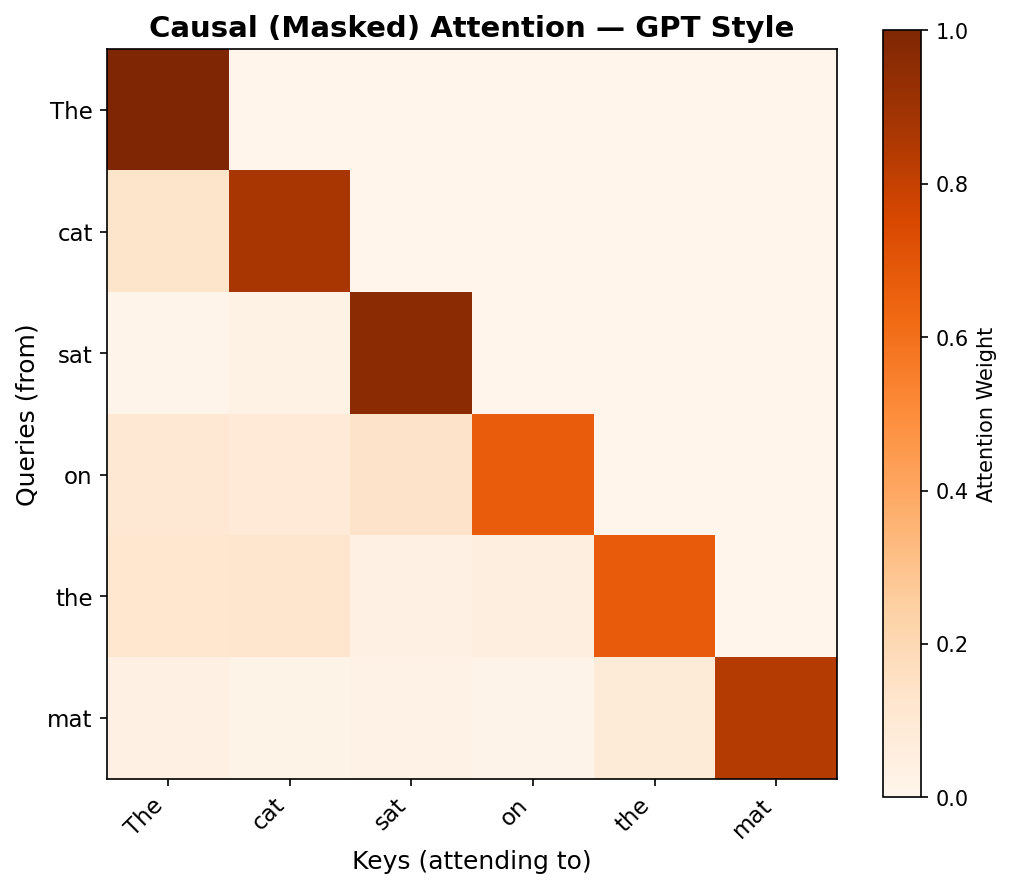
Key difference from BERT:
- Lower triangular pattern: Each token can only attend to itself and previous tokens
- No future leakage: Token at position 3 cannot see tokens 4, 5, 6...
- Why? During generation, future tokens don't exist yet!
This is implemented by masking future positions with \(-\infty\) before softmax.
BERT vs GPT: Key Differences
| BERT | GPT | |
|---|---|---|
| Architecture | Encoder-only | Decoder-only |
| Context | Bidirectional | Left-to-right (causal) |
| Pre-training | Masked LM + NSP | Next token prediction |
| Best for | Understanding (QA, NER, classification) | Generation (text completion, chat) |
Rule of thumb: BERT for analysis, GPT for generation.
BERT vs GPT: Visual Comparison
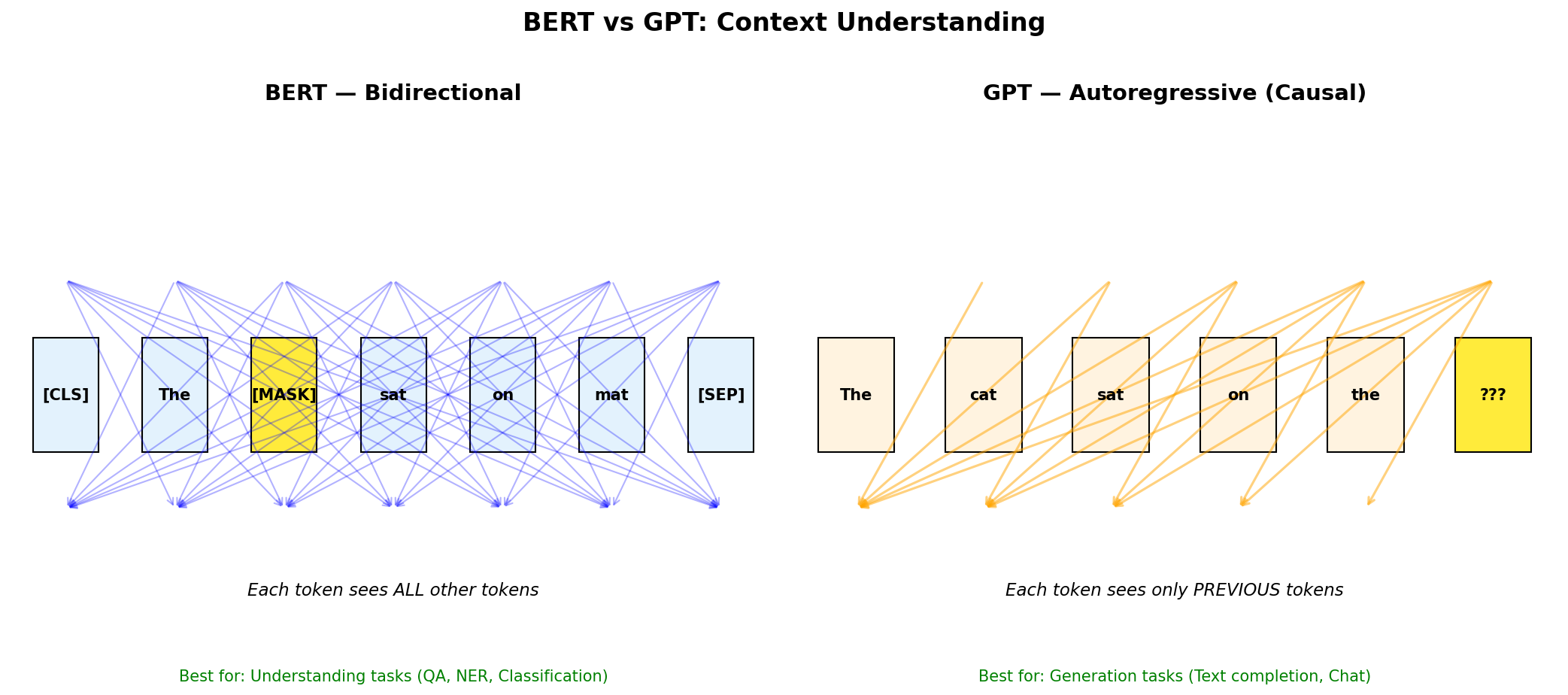
BERT (left): Every token attends to every other token — full bidirectional context for understanding.
GPT (right): Each token only sees previous tokens — perfect for text generation.
Using Pre-trained Models in Practice
The Hugging Face 🤗 Transformers library makes this easy:
from transformers import pipeline

# Sentiment analysis with BERT-based model
classifier = pipeline("sentiment-analysis")
result = classifier("I absolutely loved this movie!")
# [{'label': 'POSITIVE', 'score': 0.9998}]

# Text generation with GPT-2
generator = pipeline("text-generation", model="gpt2")
text = generator("Once upon a time", max_length=50)
# Generates a continuation...
No need to train from scratch — leverage billions of parameters!
Fine-tuning for Your Task
Add a task-specific head and train on your labeled data:
digraph finetune {
  rankdir=TB;
  node [fontsize=10, shape=box, style=rounded];

  input [label="Your Task Data\n(e.g., reviews + labels)"];
  bert [label="Pre-trained BERT\n(frozen or fine-tuned)"];
  head [label="Classification Head\n(new Linear layer)"];
  output [label="Predictions\n(positive/negative)"];

  input -> bert -> head -> output;
}
- Freeze BERT and train only the head (feature extraction).
- Or fine-tune everything with a small learning rate.
Interactive Demos & Resources
Explore how models attend to different words:
- exBERT — Visualize BERT attention heads interactively.
- BertViz — Interactive attention visualization tool.
- The Illustrated Transformer — Jay Alammar's visual guide.
- Attention? Attention! — Lilian Weng's comprehensive deep dive.
Try: Type a sentence and observe which words attend to which.
Beyond BERT & GPT
- RoBERTa: BERT with better training (no NSP, more data).
- DistilBERT: 60% smaller, 95% performance — via knowledge distillation.
- T5: Text-to-Text Transfer Transformer — everything is text generation.
- GPT-4, Claude, Gemini: Large language models at scale.
- LLaMA, Mistral: Open-weight models for research.
The field moves fast — but the fundamentals (attention, pre-training) remain the same.
Hands-On / Homework Ideas
- Use Hugging Face pipelines for sentiment analysis on custom text.
- Fine-tune a small BERT model on a classification dataset (e.g., IMDB).
- Experiment with GPT-2 text generation — try different prompts.
- Visualize attention patterns using exBERT or BertViz.
- Compare predictions from BERT vs GPT on the same input.
Summary
- Attention allows models to focus on relevant parts of a sequence.
- Transformers use self-attention for parallel, efficient processing.
- BERT (bidirectional) excels at understanding tasks.
- GPT (autoregressive) excels at text generation.
- Pre-trained models transfer knowledge to downstream tasks with minimal fine-tuning.
Next: Multi-modal AI — combining vision and language (CLIP, image captioning).