Lesson 5: Variational Autoencoders & Latent PCA

Learning Objectives

• Understand how the convolutional VAE in projects/face_autoencoder/src/model.py encodes and decodes face images.
• Explain the reparameterization trick and the \(\beta\)-ELBO loss implemented in VAELoss.
• Collect latent representations, run PCA, and use the Gradio sliders in app.py to traverse interpretable directions.

Plain Autoencoder (Deterministic)

A basic autoencoder compresses and reconstructs data without any probabilistic latent space.

digraph ae_flow {
  rankdir=LR;
  node [fontsize=11, shape=box, style=rounded];

  x      [label="Input image\nx"];
  enc    [label="Encoder\nConv / Linear layers"];
  z      [label="Latent code\nz"];
  dec    [label="Decoder\nConvTranspose / Linear"];
  x_hat  [label="Reconstruction\nx̂"];

  x -> enc -> z -> dec -> x_hat;
}
          

• Train by minimizing reconstruction loss (e.g., MSE) between \(x\) and \(\hat{x}\).
• Latent code \(z\) is a deterministic function of \(x\) with no explicit prior.
• Works well for compression and denoising, but latent space may have gaps and is not guaranteed to be smooth.

Autoencoders on MNIST / Fashion-MNIST

Before VAEs, it is useful to build intuition with a small, deterministic autoencoder on simple 28x28 images.

• Datasets: MNIST (digits) and Fashion-MNIST (clothing items).
• Goal: learn a compact latent code that can reconstruct inputs and optionally denoise simple corruptions.
• Architecture: 2–3 fully connected or convolutional layers in the encoder and a mirrored decoder.

class MnistAutoencoder(nn.Module):
    def __init__(self, latent_dim=32):
        super().__init__()
        self.encoder = nn.Sequential(
            nn.Flatten(),
            nn.Linear(28 * 28, 256), nn.ReLU(),
            nn.Linear(256, latent_dim),
        )
        self.decoder = nn.Sequential(
            nn.Linear(latent_dim, 256), nn.ReLU(),
            nn.Linear(256, 28 * 28), nn.Sigmoid(),
        )

    def forward(self, x):
        z = self.encoder(x)
        x_hat = self.decoder(z).view(-1, 1, 28, 28)
        return x_hat

We will use this style of model for the homework on MNIST and Fashion-MNIST.

Where the VAE Fits

We train a generative model that learns a smooth latent space of 64x64 RGB faces and supports interactive exploration.

digraph vae_flow {
  rankdir=LR;
  node [fontsize=12, shape=box, style=rounded, height=0.7];
  edge [penwidth=1.5];
  graph [nodesep=0.5, ranksep=0.8];

  images   [label="Input faces\n(x) [64x64x3]"];
  encoder  [label="Encoder CNN\nstrided conv blocks", style="filled,rounded", fillcolor="#e3f2fd"];
  heads    [label="Latent heads\nfc_mu & fc_logvar"];
  sample   [label="Reparameterize\nmu + sigma * eps", style="filled,rounded", fillcolor="#fff3e0"];
  decoder  [label="Decoder CNN\nConvTranspose + Tanh", style="filled,rounded", fillcolor="#e3f2fd"];
  recon    [label="Reconstruction\n~x", style="filled,rounded", fillcolor="#e8f5e9"];
  pca      [label="Latent PCA\nmetadata + sliders"];

  images -> encoder -> heads -> sample -> decoder -> recon;
  heads -> pca [style=dashed];
  sample -> pca [style=dashed];
}
          

• The encoder compresses spatial structure; latent heads model a Gaussian posterior; the decoder mirrors the encoder.
• Latent samples feed both reconstruction training and the PCA analysis used later in the app.

Encoder Anatomy

self.encoder_cnn = nn.Sequential(
    _conv_block(image_channels, base_channels),
    _conv_block(base_channels, base_channels * 2),
    _conv_block(base_channels * 2, base_channels * 4),
    _conv_block(base_channels * 4, base_channels * 8),
)

h = self.encoder_cnn(x)
h = h.view(x.size(0), -1)
              

Latent Gaussian + Reparameterization

def encode(self, x):
    h = self.encoder_cnn(x).view(x.size(0), -1)
    mu = self.fc_mu(h)
    logvar = self.fc_logvar(h)
    return mu, logvar

def reparameterize(self, mu, logvar):
    std = torch.exp(0.5 * logvar)
    eps = torch.randn_like(std)
    return mu + eps * std
              

Decoder & Reconstruction Quality

• `decoder_input` projects each latent vector back to the 4x4xC tensor inferred from the encoder.
• Three `_deconv_block` stages mirror the encoder by doubling spatial size via `ConvTranspose2d` strides.
• A final `ConvTranspose2d -> Tanh` predicts RGB pixels scaled to [-1, 1]; downstream utilities denormalize for visualization.

def decode(self, z):
    h = self.decoder_input(z)
    h = h.view(z.size(0), self.enc_channels, self.enc_spatial, self.enc_spatial)
    return self.decoder_cnn(h)
          

\(\beta\)-ELBO Loss

• Objective: maximize the Evidence Lower Bound \(\mathcal{L} = \mathbb{E}[\log p_\theta(x \mid z)] - \beta \; \mathrm{KL}(q_\phi(z \mid x) \Vert p(z))\).
• `VAELoss` uses `F.mse_loss` for the reconstruction term (faces are continuous) and a closed-form KL between diagonal Gaussians.
• Tuning \(\beta\) trades sharp reconstructions (low \(\beta\)) for more disentangled latents (high \(\beta\)).

recon_loss = F.mse_loss(output.reconstruction, target, reduction="mean")
kl_div = -0.5 * torch.mean(1 + logvar - mu.pow(2) - logvar.exp())
loss = recon_loss + beta * kl_div
          

Training Loop Helpers (training_utils.py)

Homework: Train an Autoencoder on MNIST & Fashion-MNIST

• Implement a small PyTorch autoencoder (MLP or shallow CNN) for 28x28 grayscale images, following the MnistAutoencoder pattern.
• Train on MNIST until reconstruction loss plateaus; visualize a grid of original vs reconstructed digits.
• Repeat training on Fashion-MNIST; compare what kinds of structure the model captures (edges, shapes, textures).
• Optionally add Gaussian noise to inputs and train a denoising autoencoder; report how this changes visual quality.
• Reflect: how does a deterministic autoencoder's latent space differ from the VAE latent space used in the face project?

Why Reparameterization Trick?

• Problem: sampling \(z \sim \mathcal{N}(\mu, \sigma^2)\) is non-differentiable
• Direct sampling breaks backpropagation: gradients can't flow through random operations
• Solution: separate randomness from learnable parameters

# ❌ Can't backprop through this
z = torch.normal(mu, std)
# mu and std have no gradients!

# ✅ Gradients flow through mu, std
eps = torch.randn_like(std)  # fixed noise
z = mu + eps * std
# Both mu and std are differentiable!

Key insight: \(\epsilon\) is sampled once and fixed; gradients flow through \(\mu\) and \(\sigma\).

Understanding KL Divergence

The KL term regularizes the learned posterior \(q_\phi(z \mid x)\) to match the prior \(p(z) = \mathcal{N}(0, I)\).

\[ \mathrm{KL}(q_\phi(z \mid x) \Vert p(z)) = \frac{1}{2} \sum_{i=1}^d \left( \sigma_i^2 + \mu_i^2 - 1 - \log \sigma_i^2 \right) \]

• \(\sigma_i^2 + \mu_i^2 - 1\): penalizes large means and variances (pushes toward standard normal)
• \(-\log \sigma_i^2\): prevents collapse (keeps variance from going to zero)
• Without KL: encoder could map each \(x\) to a different region → no smooth latent space
• With KL: encoder learns to use a shared, structured latent space

\(\beta\)-VAE: Controlling Disentanglement

The \(\beta\) parameter in \(\mathcal{L} = \mathbb{E}[\log p_\theta(x \mid z)] - \beta \; \mathrm{KL}(q_\phi(z \mid x) \Vert p(z))\) controls the trade-off:

Standard VAE: \(\beta = 1.0\) (balanced). \(\beta\)-VAE: \(\beta > 1\) for better disentanglement.

Reconstruction Loss: MSE vs Log(MSE) vs Perceptual

MSE Loss (Standard)

• Pixel-wise squared error: \(\|x - \hat{x}\|^2\)
• Simple, fast, differentiable
• Problem: averages out details → blurry reconstructions
• Large errors dominate gradients

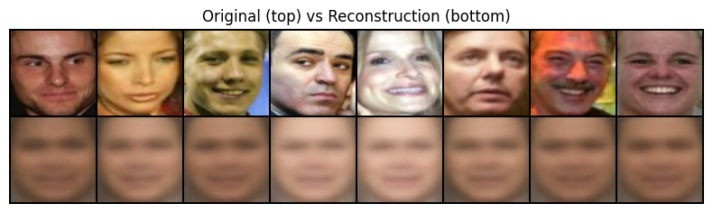
Example: MSE loss produces blurry, averaged reconstructions

recon_loss = F.mse_loss(
    output.reconstruction, 
    target
)

Log(MSE) Loss (Alternative)

• \(\log(\|x - \hat{x}\|^2 + \epsilon)\)
• Reweights gradients: \(\frac{1}{\text{MSE}} \cdot \frac{\partial \text{MSE}}{\partial \theta}\)
• Large errors contribute less; small errors contribute more
• Often produces sharper results than standard MSE
• Valid alternative that sometimes outperforms MSE

mse = F.mse_loss(output.reconstruction, target)
recon_loss = torch.log(mse + 1e-8)
# Or: loss_func = VAELoss(beta=1.0, use_log_mse=True)

Visual Comparison of VAE Losses

Different reconstruction losses change how the VAE trades sharpness vs smoothness in generated faces.

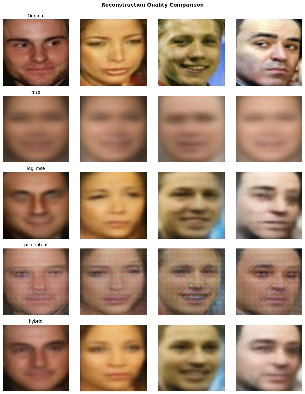
• MSE: smooth but often blurry reconstructions.
• Log(MSE): sharper details, still relatively cheap to train.
• Perceptual: most realistic faces, at the cost of extra compute.

Reconstruction Loss: Perceptual Loss

# Compare VGG features instead
recon_features = vgg(x)
target_features = vgg(target)
perceptual_loss = F.mse_loss(
    recon_features, 
    target_features
)

# Or use PerceptualVAELoss:
loss_func = PerceptualVAELoss(
    beta=1.0,
    feature_layer='relu3_3'
)

Perceptual Loss: VGG Feature Layers

Different VGG layers capture different levels of abstraction:

• relu1_2: Low-level (edges, colors) — too shallow for faces
• relu2_2: Mid-early (textures, patterns) — good detail preservation
• relu3_3: Mid-level (object parts, facial structures) — recommended for 64-96px faces
• relu4_3: High-level (semantic features) — may lose spatial detail for small images

# In PerceptualVAELoss
loss_func = PerceptualVAELoss(
    beta=1.0,
    perceptual_weight=1.0,
    mse_weight=0.1,  # Optional: hybrid approach
    feature_layer='relu3_3'  # Best for faces
)

For face images, relu3_3 balances structure preservation with detail.

Architecture Design Choices

Training Considerations

• Learning rate: Start with 1e-3 to 2e-3; VAEs can be sensitive to LR
• Batch size: Larger batches (256+) help stabilize BatchNorm and gradients
• KL annealing: Start with \(\beta=0\), gradually increase to final value (helps early training)
• Latent dimension: Too small → information bottleneck; too large → underutilized capacity
• Monitoring: Watch both reconstruction loss (quality) and KL (regularization) separately
• Early stopping: Stop when validation loss plateaus; VAEs can overfit to training faces

# Example: KL annealing
for epoch in range(epochs):
    beta = min(1.0, epoch / 50)  # Ramp up over 50 epochs
    loss_func.beta = beta
    learn.fit_one_cycle(1, lr_max=lr)

Why PCA on Latent Space?

• Interpretability: PCA finds orthogonal directions of maximum variance
• Dimensionality reduction: First few components capture most variation
• Controllable generation: Each component often corresponds to a semantic attribute (smile, pose, lighting)
• Linear interpolation: Moving along a component is smooth and predictable

Latent Space Properties

• Smoothness: Nearby points in latent space → similar faces (enabled by KL regularization)
• Completeness: Most of latent space decodes to valid faces (not just training examples)
• Interpolation: Linear paths between latents produce smooth face morphing
• Arithmetic: Can do "smiling face - neutral + angry" = new expression (if disentangled)

# Example: Interpolation
z1 = model.encode(face1)[0]  # mu for face1
z2 = model.encode(face2)[0]  # mu for face2

for alpha in [0.0, 0.25, 0.5, 0.75, 1.0]:
    z_interp = (1 - alpha) * z1 + alpha * z2
    face_interp = model.decode(z_interp)
    # Smooth morphing between faces!

Common Issues & Solutions

VAE vs Regular Autoencoder

VAEs learn a distribution over latents, enabling smooth interpolation and generation of new faces.

From Autoencoder Loss to VAE Loss

• Autoencoder objective: minimize reconstruction error only, e.g. \(L_{\text{AE}} = \mathbb{E}_{x}[\|x - \hat{x}\|^2]\).
• No explicit constraint on where latent codes \(z\) live → irregular latent space and poor samples from random \(z\).
• VAE objective: keep reconstruction term, but add a KL regularizer that pulls \(q_\phi(z \mid x)\) toward a simple prior \(p(z)\).
• This gives the Evidence Lower Bound (ELBO): \(\mathcal{L} = \mathbb{E}[\log p_\theta(x \mid z)] - \beta \, \mathrm{KL}(q_\phi(z \mid x) \Vert p(z))\).

VAE Generative Story

• Prior: choose a simple latent distribution \(p(z) = \mathcal{N}(0, I)\).
• Decoder: learn \(p_\theta(x \mid z)\) (e.g., Gaussian with mean given by a neural network) to reconstruct data from latent codes.
• Encoder: learn \(q_\phi(z \mid x)\) that maps each example to a latent Gaussian \(\mathcal{N}(\mu(x), \sigma^2(x))\).
• At test time we can either encode–decode (like an autoencoder) or sample \(z \sim p(z)\) and decode to generate new examples.

Step-by-Step: AE → VAE

Next Steps

• Reproduce the training pipeline in projects/face_autoencoder/face_autoencoder_training.ipynb and compare \(\beta\) values.
• Experiment with different latent dimensions or `base_channels`, and observe how PCA variance ratios change.
• Try PerceptualVAELoss instead of VAELoss and compare reconstruction quality.
• Extend the Gradio app with preset buttons (e.g., "add smile", "turn head") by saving curated coefficient vectors.
• Implement latent interpolation: encode two faces, interpolate in latent space, decode to see morphing.
• Optional: try ICA or t-SNE on the collected latents to contrast with PCA's linear assumptions.