Lesson 4: Data Augmentation & CNN Architectures

Learning Objectives

• Understand why and when we use data augmentation for vision models
• Recognize common augmentation operations and how to implement them in PyTorch
• Build intuition for the evolution of CNN architectures from LeNet to ResNet
• Connect CNN features to downstream tasks like object tracking

Recap: CNNs and Overfitting

• CNNs can have millions of parameters and easily memorize the training set
• Overfitting symptoms: training loss \(\downarrow\) while validation loss \(\uparrow\) or plateaus early
• We already saw regularization like Dropout and stabilization techniques like BatchNorm
• In this lesson we add weight decay and data augmentation to our toolkit

Regularization with Weight Decay

Weight decay (L2 regularization) discourages very large weights by adding a penalty to the loss.

\[ L_{\text{total}} = L_{\text{data}} + \lambda \lVert W \rVert_2^2 \]

• \(\lambda\) controls the strength of the penalty (e.g., \(10^{-4}\) or \(10^{-3}\))
• Encourages simpler models and can reduce overfitting, especially with many parameters
• In PyTorch, set weight_decay in the optimizer instead of manually modifying the loss

import torch.optim as optim

optimizer = optim.Adam(model.parameters(),
                       lr=1e-3,
                       weight_decay=1e-4)  # L2 penalty

Combine weight decay with Dropout, BatchNorm, and data augmentation for more robust CNNs.

Idea: Data Augmentation

Data augmentation creates new training examples by applying label-preserving transformations.

• Example: flipping, rotating, cropping, or color-jittering images
• We do not change the label — a rotated cat is still a cat
• Model learns to be robust to common variations (pose, lighting, small translations)
• Acts like training on a much larger dataset without collecting more images

Types of Augmentation

• Choose transforms that make sense for your data and task (e.g., avoid vertical flips for digits)

Data Augmentation Pipeline

digraph aug_pipeline {
  rankdir=LR;
  node [fontsize=13, shape=box, style=rounded, height=0.7];
  edge [penwidth=1.5];
  graph [nodesep=0.7, ranksep=0.9];

  raw   [label="Original image\n(train sample)"];
  aug   [label="Random transforms\n(flip, rotate, color jitter)", style="filled,rounded", fillcolor="#fff3e0"];
  batch [label="Augmented batch\n(x_batch, y_batch)"];
  model [label="CNN model\n(f(x; θ))", style="filled,rounded", fillcolor="#e3f2fd"];

  raw -> aug -> batch -> model;
}
          

Each epoch, the same image can look different → the model sees a stream of varied views.

PyTorch: Augmentation with torchvision.transforms

import torchvision.transforms as T

train_transform = T.Compose([
    T.RandomHorizontalFlip(p=0.5),
    T.RandomRotation(degrees=10),
    T.ColorJitter(brightness=0.2, contrast=0.2),
    T.ToTensor(),
    T.Normalize((0.1307,), (0.3081,)),  # MNIST stats
])

test_transform = T.Compose([
    T.ToTensor(),
    T.Normalize((0.1307,), (0.3081,)),
])

Apply train_transform only to training data; keep validation/test transforms deterministic.

Using Transforms in a Dataset

from torchvision import datasets
from torch.utils.data import DataLoader

train_ds = datasets.MNIST(
    root="data",
    train=True,
    download=True,
    transform=train_transform,
)

test_ds = datasets.MNIST(
    root="data",
    train=False,
    download=True,
    transform=test_transform,
)

train_loader = DataLoader(train_ds, batch_size=64, shuffle=True)
test_loader = DataLoader(test_ds, batch_size=128)

Every time train_loader samples an image, a fresh random augmentation is applied.

Choosing Augmentations Carefully

• Valid if the transform does not change the label
• Digits (MNIST): horizontal flips or 180° rotations can change a “6” into a “9” → avoid
• Natural images: flips and small rotations are usually safe
• Domain-specific tasks (medical, documents) require extra care and domain knowledge

When Does Augmentation Help Most?

• You have limited labeled data and a relatively large model
• Test-time conditions are diverse: different devices, lighting, or viewpoints
• You want robustness to small perturbations (cropping, noise, color shifts)
• Often combined with Dropout/BatchNorm and early stopping

From LeNet to Modern CNNs

Architecture design evolved, but core building blocks stayed similar.

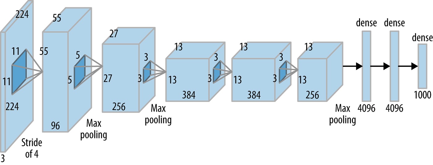
AlexNet: Bigger CNN for ImageNet

• Problem: ImageNet has millions of RGB images and 1000 classes — LeNet is too small and shallow.
• Key ideas: deeper conv stack (5 conv + 3 FC), ReLU everywhere, Dropout in fully connected layers, trained on GPUs.
• What it solved: showed CNNs can scale to large, real-world datasets and dramatically beat hand-crafted features.
• Trade-offs: large model (tens of millions of parameters), heavy compute and memory usage.

AlexNet Architecture (Diagram)

High-level view of the original AlexNet layers (input, conv / pooling blocks, fully connected head).

Architecture Sketch: LeNet vs AlexNet

LeNet vs AlexNet (Summary)

Both use conv + nonlinearity + pooling → fully connected layers; AlexNet scales this pattern up for large-scale vision.

• Why AlexNet? ImageNet is much larger and more varied than MNIST, so we need a deeper, higher-capacity CNN.
• How: more conv layers, many more channels, aggressive pooling, and heavy use of ReLU + Dropout.
• Key changes vs LeNet: supports RGB images, trains on GPUs, and scales up width/depth to handle 1000-way classification.

VGG: Deep and Simple

• Key idea: stack many \(3\times3\) conv layers instead of a few large kernels
• Pattern: \((\text{Conv} \rightarrow \text{ReLU})\) repeated 2–3 times → max pool → repeat
• Why: deeper networks capture more complex patterns; keeping blocks identical simplifies design and tuning.
• Changes vs AlexNet: replaces large, varied kernels with repeated \(3\times3\) convs, trading width for depth and regular structure.
• Downside: many parameters and heavy computation (expensive without modern accelerators).

# simplified VGG-style block
import torch.nn as nn

vgg_block = nn.Sequential(
    nn.Conv2d(64, 64, kernel_size=3, padding=1),
    nn.ReLU(),
    nn.Conv2d(64, 64, kernel_size=3, padding=1),
    nn.ReLU(),
    nn.MaxPool2d(2),  # spatial size / 2
)

Inception: Multi-Scale Features

Inception modules apply multiple filter sizes in parallel and concatenate outputs.

digraph inception_block {
  rankdir=TB;
  node [fontsize=10, shape=box, style=rounded];

  input  [label="input feature map"];
  b1_1x1 [label="1×1 conv"];
  b2_1x1 [label="1×1 conv\n(reduce)"];
  b2_3x3 [label="3×3 conv"];
  b3_1x1 [label="1×1 conv\n(reduce)"];
  b3_5x5 [label="5×5 conv"];
  b4_pool [label="3×3 max pool"];
  b4_1x1 [label="1×1 conv"];
  concat [label="concat\nchannels"];

  input -> b1_1x1 -> concat;
  input -> b2_1x1 -> b2_3x3 -> concat;
  input -> b3_1x1 -> b3_5x5 -> concat;
  input -> b4_pool -> b4_1x1 -> concat;
}
          

Network chooses useful features at multiple scales (1×1, 3×3, 5×5) in the same layer.

• Why: different objects and patterns appear at different scales; a single kernel size can miss useful structure.
• How: parallel branches with 1×1, 3×3, 5×5 convs and pooling, plus 1×1 “bottlenecks” to keep compute affordable.
• Changes vs VGG: moves from a single conv path per block to multi-branch modules that learn multi-scale features in one stage.

ResNet: Residual Connections

Residual (skip) connections help train very deep networks by making layers learn a residual correction.

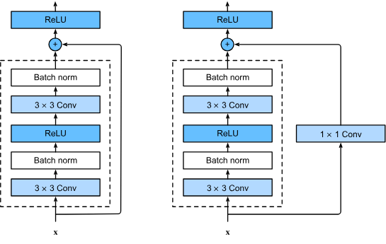
• Why: very deep plain networks are hard to train (vanishing gradients, degradation — deeper nets perform worse).
• How: each block learns a residual \(F(x)\); the skip connection lets gradients flow directly through \(x\).

ResNet: Going Deeper

Stacking many residual blocks with skip connections makes 50–100+ layer CNNs trainable in practice.

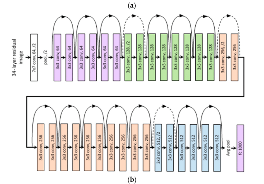
• Changes vs Inception/VGG: focuses on depth with identity shortcuts instead of complex multi-branch modules.
• Residual paths act like “highways” for gradients, reducing vanishing-gradient issues in very deep models.

Code: Simple Residual Block (PyTorch)

class BasicBlock(nn.Module):
    def __init__(self, in_ch, out_ch):
        super().__init__()
        self.conv = nn.Sequential(
            nn.Conv2d(in_ch, out_ch, 3, padding=1),
            nn.BatchNorm2d(out_ch),
            nn.ReLU(),
            nn.Conv2d(out_ch, out_ch, 3, padding=1),
            nn.BatchNorm2d(out_ch),
        )
        self.relu = nn.ReLU()

    def forward(self, x):
        out = self.conv(x)
        out = out + x  # skip connection (same shape)
        return self.relu(out)

Here the block learns a residual \(F(x)\) and adds it back to the original input \(x\) before the final ReLU.

xResNet: Inception-Inspired CNN

• xResNet variants combine residual connections with Inception-style improvements for efficiency.
• Depthwise separable convolutions: factor a standard conv into cheaper steps (per-channel spatial conv + 1×1 mixing) to reduce parameters and FLOPs.
• Batch normalization + ReLU: stabilize training and allow deeper networks.
• Global average pooling: replace large fully-connected layers with a compact pooling + small classifier head.

Depthwise Separable Convolutions

• Standard conv: every filter looks at all input channels at once (expensive: \(k \times k \times C_{in} \times C_{out}\)).
• Depthwise step: apply one \(k \times k\) filter per input channel (no channel mixing yet).
• Pointwise step: a cheap \(1 \times 1\) conv mixes channels to get the desired \(C_{out}\).
• Total cost is much lower, so we can build deeper or wider CNNs with similar compute and better accuracy.

Depthwise Separable Conv: xResNet18 Block

xResNet18-style block: depthwise + pointwise conv inside a residual (skip) connection.

digraph depthwise_sep_conv {
  rankdir=LR;
  node [fontsize=10, shape=box, style=rounded];

  input     [label="input\nfrom previous block"];
  depthwise [label="depthwise conv\nk×k per channel"];
  pointwise [label="pointwise conv\n1×1 across channels"];
  skip      [label="skip / identity\n(optional 1×1 conv)"];
  add       [label="add\n(residual + conv output)"];
  output    [label="output\nto next block"];

  input -> depthwise -> pointwise -> add -> output;
  input -> skip -> add;
}
          

Transfer Learning with CNNs

• Modern practice: start from a CNN pre-trained on a large dataset (e.g., ImageNet)
• Freeze most convolutional layers; replace and train the final classifier head
• Works well even with limited labeled data in your domain
• In this lesson we implement transfer learning with data augmentation in the companion notebook

Transfer Learning with xResNet18

• Use a pretrained xresnet18 backbone instead of training all weights from scratch on CIFAR-10.
• Phase 1 (frozen): freeze early layers and train only the new classification head for a few epochs.
• Phase 2 (fine-tune): unfreeze more layers and train with a smaller learning rate to gently adapt pretrained features.
• Helps small or medium-sized datasets achieve higher accuracy and faster convergence with less overfitting.

Switch to Notebook / Code

• Open notebooks/lesson4_data_augmentation.ipynb
• Add and visualize data augmentation for your training images
• Apply transfer learning with a pre-trained CNN (e.g., ResNet) on a smaller dataset
• Compare results with and without augmentation / fine-tuning

Image Feature Vectors

• A feature vector is a numeric representation of an image: a 1D vector \([f_1, f_2, \dots, f_d]\).
• A pretrained CNN (e.g., xresnet18) maps each image to a point in a high-dimensional space (e.g., 512-D).
• Nearby points correspond to visually or semantically similar images (e.g., similar objects, colors, textures).
• We can store these vectors and compare them instead of comparing raw pixels.

Cosine Similarity for Image Search

• Cosine similarity measures the angle between two feature vectors \(u\) and \(v\): \(\cos(\theta) = \frac{u \cdot v}{\|u\|\|v\|}\).
• Values are in \([-1, 1]\); higher values (closer to 1) mean more similar direction in feature space.
• For image retrieval: compute the feature vector of a query image and rank dataset images by cosine similarity.
• This is the core idea behind many “find similar images” and recommendation systems.

Evaluating Similarity Search

• Accuracy: fraction of predictions that are correct, \(\text{Accuracy} = \frac{TP + TN}{TP + TN + FP + FN}\).
• Precision: of the images you retrieved as “similar”, what fraction are actually relevant? \(\text{Precision} = \frac{TP}{TP + FP}\).
• Recall: of all relevant images in the dataset, what fraction did your system retrieve? \(\text{Recall} = \frac{TP}{TP + FN}\).
• For each backbone (e.g., ResNet18 vs xResNet18), compute these metrics on a small labeled subset to compare retrieval quality.

Check Your Understanding

• Why does data augmentation usually improve generalization for CNNs trained on small image datasets?
• How do depthwise separable convolutions reduce computation compared to a standard convolution?
• What does a high cosine similarity between two image feature vectors tell you about the underlying images?
• Why can transfer learning with a pretrained backbone outperform training the same architecture from scratch on CIFAR-10?

Homework

• Build a small Gradio app that takes a custom input image (file upload) and returns the most similar images from a reference set.
• Use a pretrained CNN backbone (e.g., xresnet18) to extract a feature vector for each image.
• Compute cosine similarity between the query feature vector and all reference features, and display the top-\(k\) matches with similarity scores.
• Optionally, compare at least two different backbones (e.g., ResNet18 vs xResNet18) and report precision, recall, and accuracy on a small labeled evaluation set.
• Document your design choices (feature extractor, reference dataset, normalization) and briefly discuss limitations of this approach.