Lesson 2: How Neural Networks Learn

Learning Objectives

• Explain how neural networks learn from data (forward pass, loss, gradients, optimizers)
• Understand and compare common activation functions and when to use them
• Understand regression and classification losses, including cross-entropy as “surprise”
• Understand SGD, momentum, and Adam update rules and their effect on training
• Apply these ideas by training, evaluating, and running inference on MNIST in the PyTorch notebook

Recap: Single Neuron & Activation

From Lesson 1: a single neuron computes a weighted sum, then applies an activation.

\[ z = \sum_{i=1}^d w_i x_i + b, \quad a = \sigma(z) \]

• \(x_i\): input features, \(w_i\): weights, \(b\): bias
• \(\sigma(\cdot)\): activation function (e.g., ReLU, sigmoid)
• Activation introduces nonlinearity so networks can model complex patterns

Visualization: Simple Neuron

digraph simple_neuron {
  rankdir=LR;
  node [fontsize=14];
  edge [penwidth=1.5];

  x1 [label="x₁", width=0.6];
  x2 [label="x₂", width=0.6];
  x3 [label="x₃", width=0.6];
  neuron [label="z = w·x + b\n a = σ(z)", shape=circle, style=filled, fillcolor="#e3f2fd", width=1.5];
  y [label="output a", shape=box, style="filled,rounded", fillcolor="#e8f5e9"];

  x1 -> neuron;
  x2 -> neuron;
  x3 -> neuron;
  neuron -> y;
}
          

Inputs are combined linearly into \(z\), then passed through an activation \(\sigma\) to produce output \(a\).

Activations and Learning

• Without nonlinear activations, stacked layers collapse to a single linear map
• Nonlinearities shape how gradients flow and what patterns can be learned
• Hidden layers: usually ReLU or variants (LeakyReLU, GELU)
• Output layer: choose activation to match task and loss
• Rule of thumb: ReLU in hidden layers, sigmoid or softmax at the output

ReLU in Practice

\(\mathrm{ReLU}(z) = \max(0, z)\) — standard for hidden units.

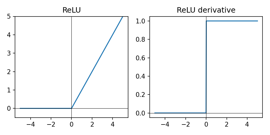
• Simple piecewise linear shape (0 for \(z \lt 0\), linear for \(z \gt 0\)); cheap to compute
• Sparse activations (many zeros) can help generalization
• Works well with modern optimizers like Adam for vision and tabular data
• If many units die (always zero), try LeakyReLU

LeakyReLU in Practice

\(\mathrm{LeakyReLU}_\alpha(z) = \max(\alpha z, z)\) with small \(\alpha \approx 0.01\).

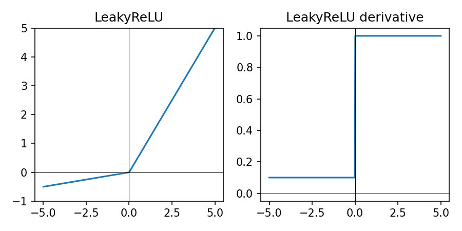
• Like ReLU but with a small negative slope for \(z \lt 0\)
• Reduces the “dying ReLU” problem by keeping gradients non-zero for negative inputs
• Useful when many ReLU units are stuck at zero during training
• Slightly more complex than ReLU but still cheap to compute

ELU in Practice

\(\mathrm{ELU}_\alpha(z) = \begin{cases} z & \text{if } z \ge 0 \\ \alpha (e^{z} - 1) & \text{if } z < 0 \end{cases}\), typically with \(\alpha = 1\).

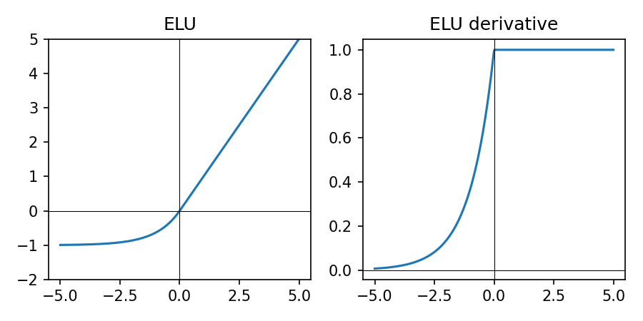
• Smooth version of ReLU: negative inputs map to negative outputs instead of exactly 0
• Can help keep activations more zero-centered and reduce bias shift
• Slightly more expensive than ReLU/LeakyReLU due to the exponential
• Less common today than ReLU/LeakyReLU but still useful to try in some vision models

GELU in Practice

\(\mathrm{GELU}(z) \approx \tfrac{1}{2} z \big(1 + \tanh\big(\sqrt{\tfrac{2}{\pi}} (z + 0.044715 z^3)\big)\big)\).

Smooth, probabilistic variant of ReLU, commonly used in transformers.

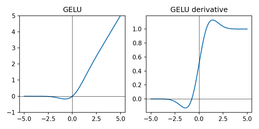
• Soft ReLU-like behavior with smooth gradients over all \(z\)
• Popular in large transformer models; more expensive than ReLU/LeakyReLU
• For small/medium models in this course, ReLU (or LeakyReLU) is usually sufficient

Sigmoid in Practice

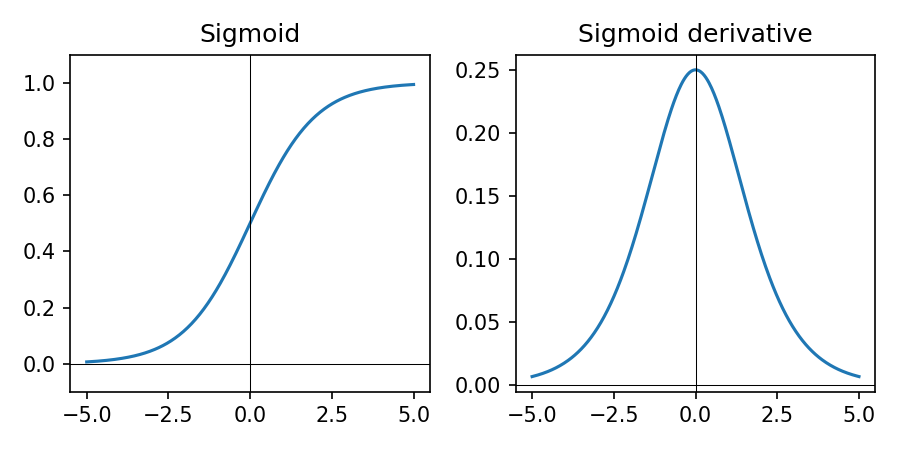
• Sigmoid squashes real-valued inputs to \((0, 1)\)
• Derivative is largest near 0 and tiny near 0 or 1 → can cause vanishing gradients when saturated
• Good for binary outputs with BCE-style losses; interpret as probability of class 1
• Avoid in deep hidden layers; prefer ReLU/LeakyReLU or GELU

Tanh in Practice

\(\tanh(z) = \frac{e^{z} - e^{-z}}{e^{z} + e^{-z}}\) — squashes to \((-1, 1)\).

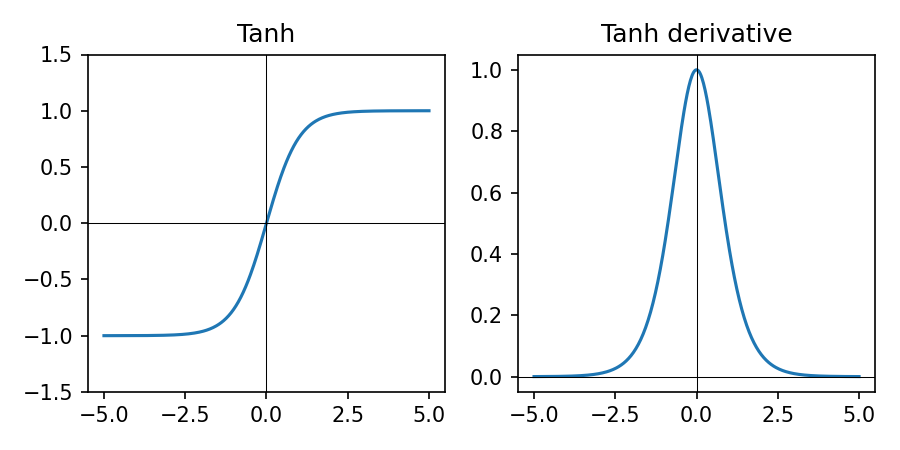
• Outputs are zero-centered, which can help optimization compared to sigmoid
• Derivative is largest near 0 and saturates (goes to 0) for large \(|z|\)
• Historically popular in RNNs; less common in modern deep nets due to saturation
• Use when you need outputs roughly in \([-1, 1]\) and can tolerate vanishing gradients

Softmax in Practice

\[ \text{softmax}_k(\mathbf{z}) = \frac{e^{z_k}}{\sum_j e^{z_j}} \]

digraph softmax_flow {
  rankdir=LR;
  node [fontsize=10];

  x1  [label="NN score\n(cat)", shape=circle];
  x2  [label="NN score\n(dog)", shape=circle];
  x3  [label="NN score\n(plane)", shape=circle];
  x4  [label="NN score\n(car)", shape=circle];

  z1  [label="10\n(cat logit)", shape=box];
  z2  [label="4\n(dog logit)", shape=box];
  z3  [label="5\n(plane logit)", shape=box];
  z4  [label="8\n(car logit)", shape=box];
  sm  [label="softmax", shape=box, style=rounded];
  p1  [label="0.873\nP(cat)"];
  p2  [label="0.002\nP(dog)"];
  p3  [label="0.006\nP(plane)"];
  p4  [label="0.119\nP(car)"];

  x1 -> z1 -> sm;
  x2 -> z2 -> sm;
  x3 -> z3 -> sm;
  x4 -> z4 -> sm;
  sm -> p1;
  sm -> p2;
  sm -> p3;
  sm -> p4;
}
          

• Converts a vector of logits \(\mathbf{z}\) into a probability distribution over classes
• Used at the output of multi-class classifiers together with cross-entropy loss

Activation Cheat Sheet

• Hidden layers: ReLU (default), LeakyReLU or ELU if many units die; GELU for transformer-style models
• Regression output: no activation (linear); optionally clamp in code if needed
• Binary classification: sigmoid output + binary cross-entropy style loss
• Multi-class (single label): logits + softmax + cross-entropy loss

From Forward Pass to Learning

• Forward pass: given weights, compute predictions \(\hat{y} = f_\theta(x)\)
• Learning: adjust parameters \(\theta\) to make predictions match labels \(y\)
• \(\theta\) collects all trainable parameters of the model (weights, biases, embeddings, etc.)
• We need: a way to measure error (loss) and a way to update \(\theta\) (optimizer)
• Training loop = repeat: forward → loss → gradients → parameter update

Diagram: Training Loop

digraph training_loop {
  rankdir=LR;
  node [shape=box, fontsize=13, style=rounded, height=0.6];
  edge [penwidth=1.5];
  graph [nodesep=0.6, ranksep=0.8];

  data      [label="Mini-batch (x, y)"];
  model     [label="Model f_θ", style="filled,rounded", fillcolor="#e3f2fd"];
  preds     [label="Predictions ŷ"];
  loss      [label="Loss L(ŷ, y)", style="filled,rounded", fillcolor="#ffcdd2"];
  grads     [label="Gradients ∂L/∂θ"];
  optimizer [label="Optimizer update\nθ ← θ - η∂L/∂θ", style="filled,rounded", fillcolor="#c8e6c9"];

  data -> model -> preds -> loss -> grads -> optimizer;
  optimizer -> model [label="updated θ", fontsize=10, style=dashed];
}
          

Key idea: the loss tells us how wrong we are; gradients tell us how to change \(\theta\).

Gradient Descent: Core Idea

We want to move parameters \(\theta\) in the direction that reduces loss.

\[ \theta_{\text{new}} = \theta_{\text{old}} - \eta \, \nabla_\theta L(\theta) \]

• \(\nabla_\theta L\): gradient — direction of steepest increase in loss
• \(\eta\): learning rate — how big each step is
• \(\theta\) typically includes all weights and biases (and any other trainable parameters) in the neural network
• Backpropagation efficiently computes these gradients layer by layer

Mini-Batch Training

• Compute loss and gradients on a small batch of examples (e.g., 64 images)
• Update parameters after each batch → faster, more memory efficient
• Noisy gradients can actually help escape poor local minima
• In PyTorch, DataLoader handles batching and shuffling

Code: Backpropagation in PyTorch

for x_batch, y_batch in data_loader:
    optimizer.zero_grad()        # reset gradients
    logits = model(x_batch)      # forward pass
    loss = loss_fn(logits, y_batch)
    loss.backward()              # backprop: compute ∂L/∂θ
    optimizer.step()             # gradient descent step on θ

This loop implements the steps: forward → loss → gradients via backward() → parameter update via optimizer.step().

Loss Functions: Measuring Error

• Loss \(L(\hat{y}, y)\) is low when predictions are good, high when they are bad
• We minimize average loss over the dataset: \(\frac{1}{N}\sum_i L(\hat{y}_i, y_i)\)
• Regression: often Mean Squared Error (MSE) or Mean Absolute Error (MAE)
• Classification: usually cross-entropy loss (works well with probabilities)

MSE Loss in Practice

Mean Squared Error for real-valued targets \(y\) and predictions \(\hat{y}\):

\[ L_{\text{MSE}} = \frac{1}{N}\sum_i (\hat{y}_i - y_i)^2 \]

• Penalizes large errors more strongly (squares the error)
• Smooth gradients make it a good default for many regression problems
• Example (target \(y = 4\)): prediction \(5 \Rightarrow \text{MSE}=1\); prediction \(8 \Rightarrow \text{MSE}=16\)

MAE Loss in Practice

Mean Absolute Error for real-valued targets \(y\) and predictions \(\hat{y}\):

\[ L_{\text{MAE}} = \frac{1}{N}\sum_i \lvert \hat{y}_i - y_i \rvert \]

• More robust to outliers: large errors are not squared
• Gradient magnitude does not grow with the size of the error
• Example (target \(y = 4\)): prediction \(5 \Rightarrow \text{MAE}=1\); prediction \(8 \Rightarrow \text{MAE}=4\)
• Consider MAE when you have many outliers or heavy-tailed noise

Binary Cross-Entropy (Sigmoid Output)

For binary labels \(y \in \{0, 1\}\) and predicted probability \(p = \hat{y}\):

\[ L_{\text{BCE}}(p, y) = -\big( y \log p + (1-y)\log(1-p) \big) \]

• Large penalty when we are confident and wrong
• Small penalty when we are confident and correct
• Works naturally with a sigmoid output in \((0,1)\)
• Interpretation: when \(y=1\), the loss is \(-\log p\); when \(y=0\), it is \(-\log(1-p)\) — in both cases this measures the model's "surprise" at the true label
• Example: \(y=1, p=0.9 \Rightarrow L \approx 0.11\); \(y=1, p=0.1 \Rightarrow L \approx 2.30\) (confident and wrong)

Multiclass Cross-Entropy (Softmax Output)

For class scores \(\mathbf{z} \in \mathbb{R}^K\) and true class index \(y \in \{0, \dots, K-1\}\):

\[ \text{softmax}_k(\mathbf{z}) = \frac{e^{z_k}}{\sum_j e^{z_j}}, \quad L(\mathbf{z}, y) = -\log \text{softmax}_{y}(\mathbf{z}) \]

• Here \(y\) is the index of the true class; we take the softmax probability at position \(y\) and apply \(-\log\) to it
• Softmax converts scores into a probability distribution over classes
• Cross-entropy encourages high probability on the correct class
• Interpretation: \(-\log p(\text{correct class})\) is the model's "surprise" — low surprise for confident, correct predictions; high surprise when it assigns low probability to the true class
• Default choice for multi-class problems like MNIST (10 digits)
• Example: if the correct class has probability \(0.8\), loss is \(-\log 0.8 \approx 0.22\); if it has probability \(0.2\), loss is \(-\log 0.2 \approx 1.61\)

Logits, Softmax, and CrossEntropyLoss

• Model output: the last linear layer returns logits (unnormalized scores), not probabilities
• nn.CrossEntropyLoss expects logits and internally applies LogSoftmax + negative log-likelihood, so do not add a softmax layer inside the model

import torch
import torch.nn as nn

logits = model(x_batch)               # shape: [batch_size, num_classes]
targets = y_batch                     # integer class labels, shape: [batch_size]

loss_fn = nn.CrossEntropyLoss()
loss = loss_fn(logits, targets)       # expects raw logits

pred_classes = logits.argmax(dim=1)   # class predictions from logits
probs = torch.softmax(logits, dim=1)  # optional: class probabilities for analysis

Training: pass logits + integer labels to CrossEntropyLoss. Inference: use argmax on logits; apply softmax only if you need explicit probabilities.

Matching Activation and Loss (PyTorch)

• Binary classification: use a single logit and BCEWithLogitsLoss (includes sigmoid)
• Multi-class classification: use logits of size K and CrossEntropyLoss (includes softmax)
• Regression: use linear outputs with MSELoss (or L1Loss for MAE)
• Always check that the model outputs and loss function expect the same shape and scale

Optimizers: How We Step

• SGD: basic gradient descent with learning rate \(\eta\)
• SGD + Momentum: smooths updates using a running average of gradients
• Adam: adaptive step sizes per-parameter + momentum (good default)
• Choice affects convergence speed and stability, not model capacity

SGD with Momentum (Update Rule)

Momentum adds a velocity term that accumulates gradients over time.

\[ v_{t} = \beta v_{t-1} + (1 - \beta)\,\nabla_\theta L_t, \quad \theta_{t+1} = \theta_t - \eta v_t \]

• \(v_t\): running average of recent gradients (velocity)
• \(\beta \in [0,1)\): momentum factor (e.g., 0.9) controlling how much history to keep
• Helps smooth noisy gradients and accelerates progress along consistent directions
• In PyTorch: torch.optim.SGD(model.parameters(), lr=..., momentum=0.9)

Adam Optimizer (Update Rule)

Adam keeps moving averages of both gradients and squared gradients.

\[ \begin{aligned} m_t &= \beta_1 m_{t-1} + (1-\beta_1)\,\nabla_\theta L_t \\ v_t &= \beta_2 v_{t-1} + (1-\beta_2)\,(\nabla_\theta L_t)^2 \\ \hat{m}_t &= \frac{m_t}{1-\beta_1^t}, \quad \hat{v}_t = \frac{v_t}{1-\beta_2^t} \\ \theta_{t+1} &= \theta_t - \eta\,\frac{\hat{m}_t}{\sqrt{\hat{v}_t} + \epsilon} \end{aligned} \]

• \(\hat{m}_t\): momentum-like term (first moment); \(\hat{v}_t\): per-parameter variance estimate (second moment)
• Adaptive step size: parameters with noisy/large gradients get smaller effective steps
• Works well out-of-the-box with defaults (\(\beta_1=0.9, \beta_2=0.999, \epsilon=10^{-8}\))
• In PyTorch: torch.optim.Adam(model.parameters(), lr=1e-3)

Optimizer Cheat Sheet (PyTorch)

• Default: Adam(model.parameters(), lr=1e-3) for many small/medium models
• When to favor SGD: very large datasets or convnets, when you can tune learning rate + momentum
• AdamW: variant of Adam with better weight decay; common for transformers

Optimizer Comparison on MNIST

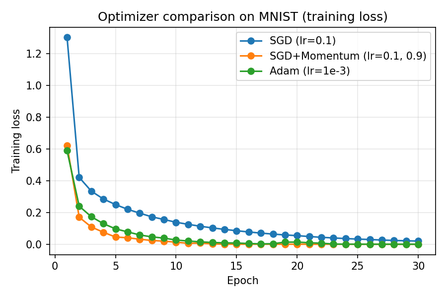
• On a small MNIST MLP, SGD with momentum and Adam reduce training loss faster than plain SGD
• Momentum accelerates progress along consistent directions; Adam adapts step sizes per parameter
• Use Adam as a strong default; switch to SGD + momentum when you can afford tuning for large convnets

Learning Rate Intuition

• Too small → very slow training, may get stuck
• Too large → loss oscillates or diverges
• Practical tip: try \(\eta \in \{1e{-3}, 3e{-3}, 1e{-4}\}\) with Adam
• Always monitor training and validation curves

Reading Training Curves

• Training loss ↓ and validation loss ↓ → learning and generalizing
• Training loss ↓, validation loss ↑ → overfitting
• Both flat → optimizer or learning rate issues
• Use curves to decide when to stop or adjust hyperparameters

Switch to Notebook: MNIST

• Now we will apply these ideas end-to-end on MNIST in the companion notebook
• Open notebooks/lesson2_Pytorch_MNIST.ipynb to walk through:
• Loading MNIST, defining the model, training, evaluation, and simple inference examples

Homework

• Train a model on the Fashion-MNIST dataset and evaluate its performance (CIFAR-10 is preferred if you have a GPU or strong CPU).
• Experiment to find a good combination of architecture, optimizer, learning rate, and number of epochs.
• Add visualizations similar to the Lesson 2 MNIST notebook: plot training and validation loss and accuracy curves.
• Run inference with your best model on a new image captured with a camera and analyze the prediction.