Lesson 1 — From Regression to Deep Learning

Lesson 1: From Regression to Deep Learning

Learning Objectives

Why linear models fail on complex data
How layers + activations extend regression
Visualize decision boundaries forming
Forward pass intuition with minimal math

Why Regression Isn’t Enough

Recall logistic regression decision boundaries
Curved datasets (circles, spirals) break linear separability
Prompt: “How could we bend this decision line?”

Notation

Input vector: \(\mathbf{x} \in \mathbb{R}^d\)
Weights: \(\mathbf{w} \in \mathbb{R}^d\), bias: \(b \in \mathbb{R}\)
Activation (nonlinearity): \(\sigma(\cdot)\) e.g., ReLU, sigmoid

Tip: hidden layers typically use ReLU; outputs use sigmoid for binary classification.

Single Neuron (Scalar Output)

Linear combination + nonlinearity:

\[ \hat{y} = \sigma\big( \mathbf{w}^\top \mathbf{x} + b \big) \]

Without \(\sigma\), this is just linear regression/logistic logit.

Shapes: \(\mathbf{x}\in\mathbb{R}^d\), \(\mathbf{w}\in\mathbb{R}^d\), \(b\in\mathbb{R}\), \(\hat{y}\in\mathbb{R}\). Common \(\sigma\): ReLU, tanh, sigmoid.

Neuron + Bias Intuition

Linear part: z = w · x + b
Activation: a = σ(z) adds nonlinearity
Bias b moves the decision threshold
Layers stack these simple units

Diagram: Single Neuron


digraph neuron {
  rankdir=LR;
  node [shape=circle, fontsize=14, width=1.0];
  edge [penwidth=1.5];

  x1 [label="x₁"];
  x2 [label="x₂"];
  x3 [label="x₃"];
  h  [label="σ(w·x + b)", width=1.5];

  x1 -> h;
  x2 -> h;
  x3 -> h;
}

Multiple inputs are combined into a single neuron that applies σ to \(w \cdot x + b\).

ReLU Activation

\(\mathrm{ReLU}(z) = \max(0, z)\) — default for hidden layers.

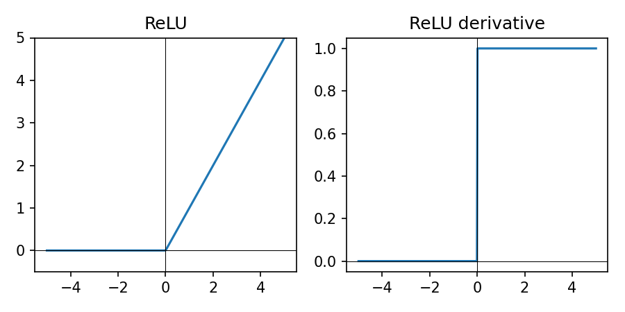
Zero for negative inputs, linear for positive
Keeps computation simple and fast
Works well as a default for hidden layers

Sigmoid Activation

\(\sigma(z) = \frac{1}{1 + e^{-z}}\) — used for binary outputs.

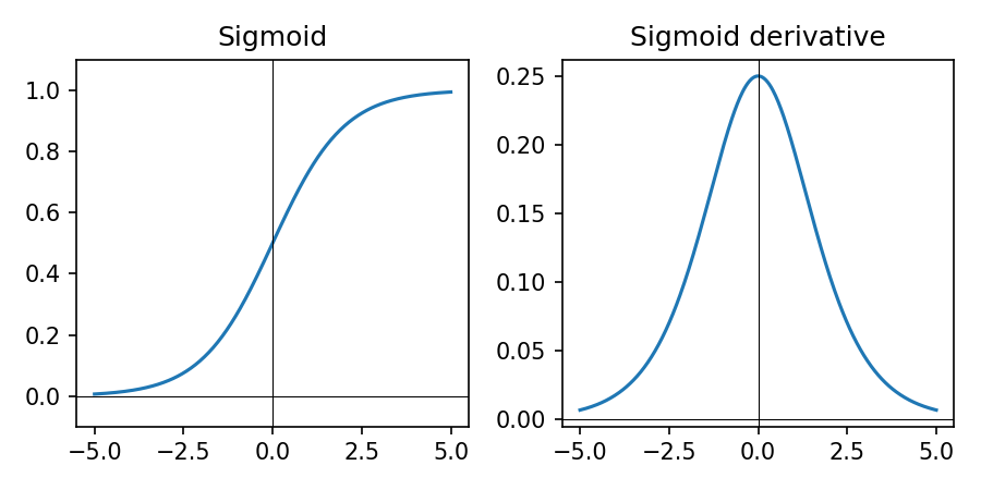
Maps any real number to (0, 1)
Interpretable as probability for binary class
Used on the final neuron in this lesson

Layer (Vector Form)

Compute multiple neurons at once:

\[ \mathbf{a}^{(1)} = \sigma\big( \mathbf{W}^{(1)} \mathbf{x} + \mathbf{b}^{(1)} \big) \]

\(\mathbf{W}^{(1)} \in \mathbb{R}^{m\times d}\) maps input to \(m\) hidden units.

Shapes: \(\mathbf{b}^{(1)}\in\mathbb{R}^m\), \(\mathbf{a}^{(1)}\in\mathbb{R}^m\). \(\sigma\) applies elementwise.

Two-Layer Network

Compose layers to get flexible decision boundaries:

\[ \hat{y} = \sigma^{(2)}\!\big( \mathbf{W}^{(2)} \, \sigma^{(1)}( \mathbf{W}^{(1)}\mathbf{x} + \mathbf{b}^{(1)} ) + \mathbf{b}^{(2)} \big) \]

Each layer: linear map + nonlinearity. Stacking learns features of features.

Shapes: hidden size \(m\), output size \(k\). \(\mathbf{W}^{(2)}\in\mathbb{R}^{k\times m}\), \(\mathbf{b}^{(2)}\in\mathbb{R}^k\), \(\hat{y}\in\mathbb{R}^k\). Typical in this lesson: \(\sigma^{(1)}=\)ReLU, \(\sigma^{(2)}=\)sigmoid.

Diagram: Two-Layer Network


digraph two_layer {
  rankdir=LR;
  node [shape=circle, fontsize=14, width=0.8];
  edge [penwidth=1.5];
  graph [nodesep=0.5, ranksep=1.0];

  subgraph cluster_input {
    label="Inputs";
    color="white";
    x1 [label="x₁"];
    x2 [label="x₂"];
  }

  subgraph cluster_hidden {
    label="Hidden layer (ReLU)";
    style=filled; fillcolor="#f5f5f5";
    h1 [label="h₁"];
    h2 [label="h₂"];
    h3 [label="h₃"];
  }

  subgraph cluster_output {
    label="Output";
    color="white";
    y [label="ŷ"];
  }

  x1 -> h1; x1 -> h2; x1 -> h3;
  x2 -> h1; x2 -> h2; x2 -> h3;
  h1 -> y;  h2 -> y;  h3 -> y;
}

Inputs feed into hidden units, which then feed into the output neuron.

Forward Pass — Step by Step

Compute each layer’s z = W·x + b
Apply activation a = σ(z)
Feed a into next layer
Final output → prediction

We’ll worry about learning (backprop) next lesson.

Key Themes

Linear part learns weighted combinations; bias shifts thresholds
Nonlinearity lets boundaries bend (beyond any single line)
Depth composes simple units into complex patterns

Interactive Demo (TF Playground)

Select circular or spiral dataset
No hidden layers → poor separation
1 hidden layer (8) → improvement
2 layers (8+8) → complex shapes classified
Tune activations, learning rate, noise

Discuss: Why deeper → better patterns? What might each neuron learn?

Open TensorFlow Playground

Mini Hands-On

Implement the idea in PyTorch on synthetic 2D points.

import torch
import torch.nn as nn

model = nn.Sequential(
  nn.Linear(2, 8),
  nn.ReLU(),
  nn.Linear(8, 8),
  nn.ReLU(),
  nn.Linear(1, 1),
  nn.Sigmoid(),
)
# optimizer = torch.optim.Adam(model.parameters(), lr=1e-3)
# loss_fn = nn.BCELoss()
# training loop ...

Plot decision regions; relate to Playground behavior.

Code: Make a 2D Dataset

# Option A: use scikit-learn (concise)
from sklearn.datasets import make_circles
import numpy as np

X, y = make_circles(n_samples=1000, factor=0.5, noise=0.1, random_state=0)
X = X.astype('float32')
y = y.astype('float32')

# Option B: quick NumPy spiral (for the curious)
def make_spiral(n=500, noise=0.2):
    n2 = n//2
    t = np.linspace(0, 2*np.pi, n2)
    r = np.linspace(0.2, 1.0, n2)
    x1 = np.c_[r*np.cos(t), r*np.sin(t)] + noise*np.random.randn(n2,2)
    x2 = np.c_[-r*np.cos(t), -r*np.sin(t)] + noise*np.random.randn(n2,2)
    Xs = np.vstack([x1, x2]).astype('float32')
    ys = np.r_[np.zeros(n2), np.ones(n2)].astype('float32')
    return Xs, ys

Code: Train and Evaluate (PyTorch)

import torch
import torch.nn as nn

X_t = torch.from_numpy(X)
y_t = torch.from_numpy(y).unsqueeze(1)

model = nn.Sequential(
    nn.Linear(2, 8),
    nn.ReLU(),
    nn.Linear(8, 8),
    nn.ReLU(),
    nn.Linear(8, 1),
    nn.Sigmoid(),
)
optimizer = torch.optim.Adam(model.parameters(), lr=1e-3)
loss_fn = nn.BCELoss()

for epoch in range(20):
    optimizer.zero_grad()
    preds = model(X_t)
    loss = loss_fn(preds, y_t)
    loss.backward()
    optimizer.step()

print('Final training loss:', float(loss))

Expect validation accuracy to improve over epochs; details next lesson.

Code: Plot Decision Regions

import numpy as np, matplotlib.pyplot as plt
import torch

xx, yy = np.meshgrid(np.linspace(X[:,0].min()-0.5, X[:,0].max()+0.5, 200),
                     np.linspace(X[:,1].min()-0.5, X[:,1].max()+0.5, 200))
grid = np.c_[xx.ravel(), yy.ravel()].astype('float32')
with torch.no_grad():
    grid_t = torch.from_numpy(grid)
    probs = model(grid_t).detach().numpy().reshape(xx.shape)

plt.figure(figsize=(5,4))
plt.contourf(xx, yy, probs, levels=20, cmap='RdBu', alpha=0.6)
plt.scatter(X[:,0], X[:,1], c=y, cmap='RdBu', edgecolor='k', s=12)
plt.title('Decision regions')
plt.show()

Relate the learned boundary to the Playground visuals.

Wrap-Up

Neuron = regression + nonlinearity on top
Layers stack neurons to learn features of features
Depth + activations bend decision boundaries into complex shapes

Homework:

In the spirals notebook, recreate one of the Playground experiments (spirals or circles).
Try at least two different architectures.
Find the deepest network (most layers) that uses the fewest units but still fits the data.
Find the shallowest network (fewest layers) that uses the fewest units but still fits the data.

Next time: how networks actually learn these weights using loss functions and gradient descent.